Given a connection  on a manifold, along with any vector basis
  , the connection coefficients are:
![\[ \Gamma_{\mu\nu}^{\hphantom{\mu\nu}\sigma} := \langle\nabla_\mu\mathbf e_\nu,\mathbf e^\sigma\rangle. \]](http://cmaclaurin.com/cosmos/wp-content/ql-cache/quicklatex.com-0da3696c8ef5490c24c4ced6dac4df8f_l3.png "Rendered by QuickLaTeX.com")
[For the usual connection based on a metric, these are called Christoffel symbols. On rare occasions some add “…of the second kind”, which we will interpret to mean the component of the output is the only raised index. Also the coefficients may be packaged into Cartan’s connection 1-forms, with components  , as introduced in the previous article. Hence raising or lowering indices on the connection forms is the same problem.]
In our convention, the first index specifies the direction  of differentiation, the second is the basis vector (field) being differentiated, and the last index is for the component of the resulting vector. We use the same angle bracket notation for the metric scalar product, inverse metric scalar product, and the contraction of a vector and covector (as above; and this does not require a metric).
This unified notation is very convenient for generalising the above connection coefficients to any variant of raised or lowered indices, as we will demonstrate by examples. We will take such variants on the original equation as a definition, then the relation to the original  variant will be derived from that.
[Regarding index placement and their raising and lowering, I was formerly confused by this issue, in the case of non-tensorial objects, or using different vector bases for different indices. For example, to express an arbitrary frame in terms of a coordinate basis, some references write the components as  , as blogged previously. The Latin index is raised and lowered using the metric components in the general frame
  , whereas for the Greek index the metric components in a coordinate frame
  are used. However while these textbook(s) gave useful practical formulae, I did not find them clear on what was definition vs. what was derived. I eventually concluded the various indices and their placements are best treated as a definition of components, with any formulae for swapping / raising / lowering being obtained from that.]
The last index is the most straightforward. We define:  , with all indices lowered. These quantities are the overlaps between the vectors
  and
and  . [Incidentally we could call them the “components” of , if this vector is decomposed in the alternate vector basis
  . After all, for any vector,
  , which may be checked by contracting both sides with
  . ] To relate to the original
  s, note:
![\[ \Gamma_{\mu\nu\tau} = \langle\nabla_\mu\mathbf e_\nu,\mathbf e^\sigma g_{\sigma\tau}\rangle = \langle\nabla_\mu\mathbf e_\nu,\mathbf e^\sigma\rangle g_{\sigma\tau} = \Gamma_{\mu\nu}^{\hphantom{\mu\nu}\sigma}g_{\sigma\tau}, \]](http://cmaclaurin.com/cosmos/wp-content/ql-cache/quicklatex.com-1e8dc7263a128cfd70916ce655732f69_l3.png "Rendered by QuickLaTeX.com")
using linearity. Hence this index is raised or lowered using the metric, as familiar for an index of a tensor. We could say it is a “tensorial” index. The output of the derivative is just a vector, after all. The  have been called “Christoffel symbols of the first kind”.
The first index is also fairly straightforward. We define a raised version by:  . However, this begs the question of what the notation ‘
 ’ means. The raised index suggests
  , which is a covector, but we can take its dual using the metric (assuming there is one). Hence
  is a sensible definition, or for an arbitrary covector,
  . (For those not familiar with the notation,
  is simply the vector with components
  .)
.)
These duals are related to the vectors of the original basis by:  , where
  are still the inverse metric components for the original basis. Hence
  , by the linearity of this slot. In terms of the coefficients,
  , hence the first index is also “tensorial”.
Finally, the middle index has the most interesting properties for raising or lowering. Let’s start with a raised middle index and lowered last index:  . This means it is now a covector field which is being differentiated, and the components of the result are peeled off. For their relation to the original coefficients, note firstly
  , since these bases are dual. These are constants, hence their gradients vanish:
![\[ 0 = \nabla_\mu \langle\mathbf e^\sigma,\mathbf e_\nu\rangle = \langle\nabla_\mu\mathbf e^\sigma,\mathbf e_\nu\rangle + \langle\mathbf e^\sigma,\nabla_\mu\mathbf e_\nu\rangle. \]](http://cmaclaurin.com/cosmos/wp-content/ql-cache/quicklatex.com-0f37b17e9f5fc89208a9b894a85bb478_l3.png "Rendered by QuickLaTeX.com")
[The second equality is not the metric-compatibility property of some connections, despite looking extremely similar in our notation. No metric is used here. Rather, it is a defining property of the covariant derivative; see e.g. Lee 2018  Prop. 4.15. But no doubt these defining properties are chosen for their “compatibility” with the vector–covector relationship.]
Hence  . Note the order of the last two indices is swapped in this expression, and their “heights” are also changed. (I mean, it is not just that
  and
and  are interchanged.) This relation is antisymmetric in some sense, and looks more striking in notation which suppresses the first index. Connection 1-forms (can) do exactly that:
  .
.
Note this is not the well-known property for an orthonormal basis, which is  using our conventions. Both equalities follow from conveniently chosen properties of bases: the dual basis relation in the former case, and orthonormality of a single basis in the latter. Our relation holds in any basis, and does not require a metric. But both relations are useful — they just apply to different contexts.
To isolate the middle index as the only one changed, raise the last index again:  . Only now have we invoked the metric, in our discussion of the middle index.
The formula has an elegant simplicity. However at first it didn’t feel right to me as the sought-after relation. We are accustomed to tensors, where a single index is raised or lowered independently of the others. However in this case the middle index describes a vector which is differentiated, and differentiation is not linear (for our purposes here), but obeys a Leibniz rule. (To be precise, it is linear over sums, and multiplication by a constant scalar. It is not linear under multiplication by an arbitrary scalar. Mathematicians call this  -linear but not
  -linear.)
The formula could be much worse. Suppose we replaced the original equation with an arbitrary operator, and defined raised and lowered coefficients similarly. Assuming the different variants are related somehow, then in general each could depend on all coefficients from the original variant, for example:  , for some functions
  with 3 × 2 = 6 indices.
Much of the material here is not uncommon. In differential geometry it is well-known the connection coefficients are not tensors. And it is not rare to hear that in fact two of their indices do behave tensorially. But I do not remember seeing a clear definition of what it means to raise or lower any index, in the literature. (Though the approach in geometric algebra, of using two distinct vector bases and  , is similar. This requires a metric, and gives a unique interpretation to raising and lowering indices. But in fairness, most transformations we have described also require a metric.) Most textbooks probably do not define different variants of the connection forms, although I have not investigated this much at present.
Finally, it is easy to look back and say something is straightforward. But not when your attention is preoccupied with grasping the core aspects of a new thing, not its more peripheral details. When I was first learning about connection forms, it was not at all clear whether you could raise or lower their indices. Because the few references I consulted didn’t mention this at all, to me it felt like it should be obvious. But it is not obvious, and demands careful consideration, even though some results are familiar ideas in a new context.
 , which are called Christoffel symbols in the special case of a metric connection.
 . This decomposes the gradient of one basis vector field in terms of all the basis vectors. In fact, this gradient is expressed in totality by the total covariant derivative
  … For each fixed value of
  from the connection in the usual sense). I will write more on this in the future.
 evaluates in detail. I certainly appreciate the modern curvature-only view for what it affirms, just not what it denies.
 . In our universe, matter forms a “cosmic web”, which includes filaments with a heavy “node” at the end — a cluster or supercluster. On the other hand, cosmic “voids” are vast regions containing less matter than average. Over time, the matter clumps further, while the voids grow larger and sparser.
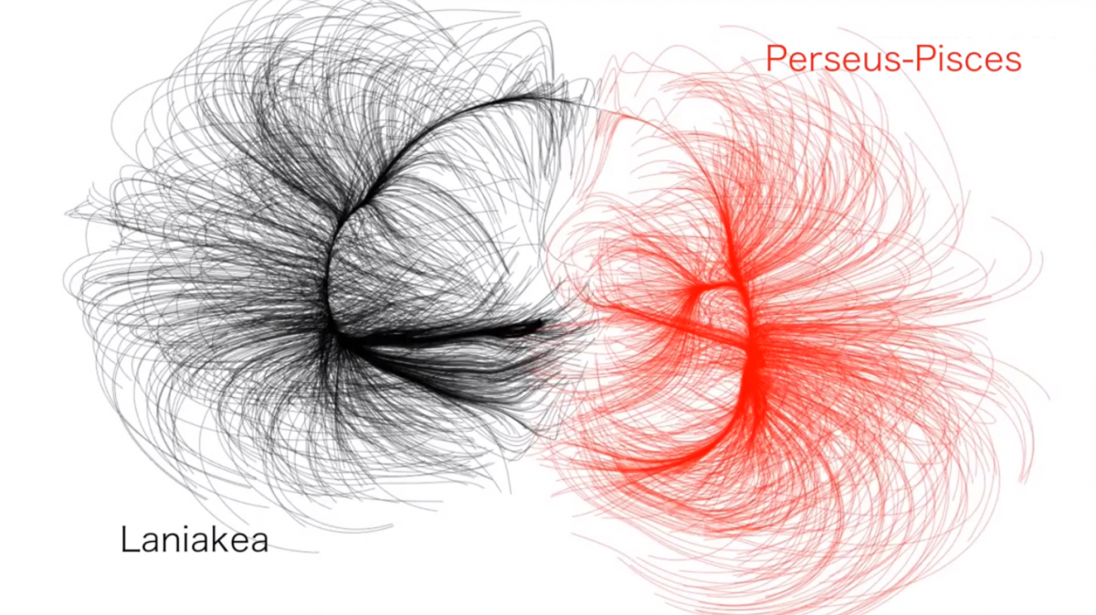
 . This is normally understood as an “internal symmetry”. But Hestenes has a remarkable proposal to interpret it geometrically in spacetime itself, using tangent vectors and bivectors formed from them, in a
  . So we seek an analogue of this structure in Minkowski spacetime. Choose an orthonormal basis:
  etc. Hestenes defines the bivectors
  ,
,  and
and  . This notation uses the geometric product, but in this case the vectors are orthogonal, so the result is just wedge products, e.g.
  . Together, the scalar and pseudoscalar parts from the geometric algebra form a subalgebra which is isomorphic to
  , the underlying field for the vector space
  (or maybe some subgroup), hence these spacetime “rotations” include both boosts and spatial rotations. Then
  encodes a boost in the
  -direction, combined with a rotation about the
  , the rotations on a 6-dimensional real space. Specifically, those which preserve the structure of the complex axes, relative to one another. However in our case these are not spacetime rotations, but act on the space of bivectors. This is quite abstract, and I envision making illustrations in future work. But just as a 2D rotation changes the
  -components of a vector, these
  and so on). Returning to
  R
R G
G R
R G
G R
R \mathfrak{su}(3)
 SU(3)
SU(3) SU(3)
SU(3) \mathfrak{su}(3)
 \mathfrak{su}(3)
 \epsilon
 R\wedge_{\mathbb C}G\wedge_{\mathbb C}B$ is valid. The wedge here is not the one acting on tangent vectors, but “complex vectors” which for us are basically bivectors. Intuitively, the “complex trivector” fills all directions of (real) bivector space. Just like the 4-volume element formed from vectors fills all spacetime directions (within a tangent space at a point, that is).
![\[ \boldsymbol\omega_\mu^{\hphantom\mu\nu} = \omega_{\mu\hphantom\nu\tau}^{\hphantom\mu\nu}\mathbf e^\tau, \qquad\qquad \boldsymbol\omega^\nu_{\hphantom\nu\mu} = \omega^\nu_{\hphantom\nu\mu\tau}\mathbf e^\tau, \]](http://cmaclaurin.com/cosmos/wp-content/ql-cache/quicklatex.com-f397e1fbf79d43687701700aa42670d2_l3.png "Rendered by QuickLaTeX.com")
![\[ \nabla_\sigma\mathbf e_\mu = \langle\nabla_\sigma\mathbf e_\mu,\mathbf e^\tau\rangle\,\mathbf e_\tau = \omega_{\mu\hphantom\tau\sigma}^{\hphantom\mu\tau}\mathbf e_\tau. \]](http://cmaclaurin.com/cosmos/wp-content/ql-cache/quicklatex.com-2d5e1b1e197351d1ed7f9e679381e304_l3.png "Rendered by QuickLaTeX.com")
 ‘. But can check it holds by contracting both sides with
  . Similarly for the covector gradients,
![\[ \nabla_\sigma\mathbf e^\nu = \langle\nabla_\sigma\mathbf e^\nu,\mathbf e_\tau\rangle\,\mathbf e^\tau = \omega^\nu_{\hphantom\nu\tau\sigma}\mathbf e^\tau = -\omega_{\tau\hphantom\nu\sigma}^{\hphantom\tau\nu}\mathbf e^\tau. \]](http://cmaclaurin.com/cosmos/wp-content/ql-cache/quicklatex.com-21127b0f5cf22f54c65756c7ef1ccf83_l3.png "Rendered by QuickLaTeX.com")
 . Because: substitute
  into the left slot (in our convention) of both sides. The RHS becomes:
  , by linearity of this slot. Now, apply this identity to
 ![\[ \nabla\mathbf e_\mu = \mathbf e^\sigma\otimes\nabla_\sigma\mathbf e_\mu = \omega_{\mu\hphantom\tau\sigma}^{\hphantom\mu\tau}\mathbf e^\sigma\otimes\mathbf e_\tau = \boldsymbol\omega_\mu^{\hphantom\mu\tau}\otimes\mathbf e_\tau. \]](http://cmaclaurin.com/cosmos/wp-content/ql-cache/quicklatex.com-8f2df818e811d8acf1ea5b7f97bb442a_l3.png "Rendered by QuickLaTeX.com")
![\[\begin{split} \nabla\mathbf e^\nu &= e^\sigma\otimes\nabla_\sigma\mathbf e^\nu = \omega^\nu_{\hphantom\nu\tau\sigma}\mathbf e^\sigma\otimes\mathbf e^\tau = -\omega_{\tau\hphantom\nu\sigma}^{\hphantom\tau\nu}\mathbf e^\sigma\otimes\mathbf e^\tau \\ &= \boldsymbol\omega^\nu_{\hphantom\nu\tau}\otimes\mathbf e^\tau = -\boldsymbol\omega_\tau^{\hphantom\tau\nu}\otimes\mathbf e^\tau. \end{split}\]](http://cmaclaurin.com/cosmos/wp-content/ql-cache/quicklatex.com-9faf56c751b9f2cc0c5b5ad6fee9bd9e_l3.png "Rendered by QuickLaTeX.com")
![\[\begin{split} d(\mathbf e^\nu) &= \boldsymbol\omega^\nu_{\hphantom\nu\sigma}\wedge\mathbf e^\sigma = \omega^\nu_{\hphantom\nu\sigma\tau}\mathbf e^\tau\wedge\mathbf e^\sigma = -\omega^\nu_{\hphantom\nu\sigma\tau}\mathbf e^\sigma\wedge\mathbf e^\tau \\ &= \omega_{\sigma\hphantom\nu\tau}^{\hphantom\sigma\nu}\mathbf e^\sigma\wedge\mathbf e^\tau. \end{split}\]](http://cmaclaurin.com/cosmos/wp-content/ql-cache/quicklatex.com-b93a68da7af62887c0b6ec1cf1a7a72c_l3.png "Rendered by QuickLaTeX.com")
 are one way to express a connection
  are more familiar and achieve the same purpose, but package the information differently. Connection forms are part of Cartan’s efficient and elegant “moving frames” approach to derivatives and curvature.
 , where
  for the contraction between a vector and covector, which is not uncommon in the literature. The unified notation with the metric scalar product is convenient, although it is sometimes worth reminding oneself that no metric is needed in this particular case.) To find the components, substitute basis vectors
  :
:![\[ \omega_{\mu\hphantom\nu\sigma}^{\hphantom\mu\nu} := \boldsymbol\omega_\mu^{\hphantom\mu\nu}(\mathbf e_\sigma) = \langle\nabla_\sigma\mathbf e_\mu,\mathbf e^\nu\rangle =: \Gamma_{\sigma\mu}^{\hphantom{\sigma\mu}\nu}, \]](http://cmaclaurin.com/cosmos/wp-content/ql-cache/quicklatex.com-d5fddf068b3b2393d8df910a2ab6e05f_l3.png "Rendered by QuickLaTeX.com")
 as usual. Hence with our conventions, the
  -index specifies which basis vector field is being differentiated,
  for our expression — which swaps the index order.)
![\[ \omega\indices^\nu_{\hphantom\nu\mu\sigma} := \boldsymbol\omega^\nu_{\hphantom\nu\mu}(\mathbf e_\sigma) := \langle\nabla_\sigma\mathbf e^\nu,\mathbf e_\mu\rangle = -\langle\nabla_\sigma\mathbf e_\mu,\mathbf e^\nu\rangle = -\omega_{\mu\hphantom\nu\sigma}^{\hphantom\mu\nu}. \]](http://cmaclaurin.com/cosmos/wp-content/ql-cache/quicklatex.com-27ef19a830d62d9e98a93fea6871076a_l3.png "Rendered by QuickLaTeX.com")
![\[ \boldsymbol\omega_\mu^{\hphantom\mu\nu} = -\boldsymbol\omega^\nu_{\hphantom\nu\mu}. \]](http://cmaclaurin.com/cosmos/wp-content/ql-cache/quicklatex.com-401382997b6ad9a63a20ec0bfb60ae95_l3.png "Rendered by QuickLaTeX.com")
![\[ 0 = \nabla_\sigma\langle\mathbf e_\mu,\mathbf e^\nu\rangle = \langle\nabla_\sigma\mathbf e_\mu,\mathbf e^\nu\rangle + \langle\mathbf e_\mu,\nabla_\sigma\mathbf e^\nu\rangle. \]](http://cmaclaurin.com/cosmos/wp-content/ql-cache/quicklatex.com-832cdb5ac5b43f58a1f9bede19948998_l3.png "Rendered by QuickLaTeX.com")
 is constant, so its gradient vanishes. The second equality follows from the defining properties of the covariant derivative, i.e. the extension of the connection to covectors and other tensors (e.g. Lee 2018
  . The Latin index is raised and lowered using the metric components in the arbitrary frame, whereas the Greek index uses the metric components in the coordinate frame. However textbooks were not clear on what was definition vs. what was derived, I thought. I eventually concluded the various indices and their placements are best treated as a definition of components, with any formulae for swapping/raising/lowering being obtained from that.]
 , in terms of our notation. I did not see how to prove this, so initially I just copied and affirmed it. But I am now updating this 6 months later, and I realise it is only true for a metric of Riemannian signature. Sorry about that.
 leads to
  . Multiply both sides by
  and sum, which gives:
 . On the LHS, this raised the second index, which is tensorial or “linear”. But on the RHS, the first index doesn’t obey the tensorial rule. (See the next article I would write on
  . Now apply orthonormality again, so the sum collapses to
  , hence:
![\[ \boldsymbol\omega_\mu^{\hphantom\mu\nu} = -\eta_{\mu\mu}\eta_{\nu\nu}\,\boldsymbol\omega_\nu^{\hphantom\nu\mu}. \]](http://cmaclaurin.com/cosmos/wp-content/ql-cache/quicklatex.com-4cfe1bdd90f00e5b6ca2a839c19a0fab_l3.png "Rendered by QuickLaTeX.com")
 .
. , whereas a covector has a lowered index:
  . Similarly the dual to
  , using the metric, is the covector with components denoted
  say; while the dual to
  is the vector with components
  .
. . Similarly, the component notation
  . These bases are taken to be dual to one another (in the sense of bases), meaning:
  . We also have
  and
and  , where as usual
  and
and  . (The “sharp” and “flat” symbols are just a fancy way to denote the dual. This is called the musical isomorphism.)
 . This gives a different decomposition than in the previous paragraph. Curiously, this expression contains a raised component index, even though it describes a covector. For each index value
  is a different decomposition of the vector
  . It describes a vector, despite using a lowered component index. Using the metric, the two vector bases are related by:
  .
. . (While
 . In the diagram we index the vectors by colour, rather than the typical 1, 2, and 3. Rather than using a co-basis of covectors as in the standard modern approach, we take both bases to be made up of vectors. Note for example, the red vector on the right is orthogonal to the blue and green vectors on the left. (I made up the directions when plotting, so don’t expect everything to be quantifiably correct.) Arguably “inverse basis” would be the best name. Finally I would prefer to start from this picture, as it is simple and intuitive, rather than start with covectors and musical isomorphisms. Maybe next time I will be brave enough.
 , which describes an orthogonal matrix. While admittedly the paper is mostly abstract algebra, he is also motivated by geometry. In §3 he mentions that the equation for a surface is “transformed” under a change of [Cartesian] coordinates, including the case where the coordinate origins coincide. We recognise this (today, at least) as a rotation, possibly combined with a reflection. Euler also mentions “angles” (§4 and later), which is clearly geometric language.
![\[\begin{tabular}{|c|c|c|}\hline $\frac{p^2+q^2+r^2+s^2}{u}$ & $\frac{2(qr+ps)}{u}$ & $\frac{2(qs-pr)}{u}$ \\ \hline $\frac{2(qr-ps)}{u}$ & $\frac{p^2-q^2+r^2-s^2}{u}$ & $\frac{2(pq+rs)}{u}$ \\ \hline $\frac{2(qs+pr)}{u}$ & $\frac{2(rs-pq)}{u}$ & $\frac{p^2-q^2-r^2+s^2}{u}$ \\ \hline\end{tabular},\]](http://cmaclaurin.com/cosmos/wp-content/ql-cache/quicklatex.com-8a820b1a5889a514cf73584ad468f584_l3.png "Rendered by QuickLaTeX.com")
 . (I have copied the style which Euler uses in some subsequent examples.) By choosing rational values of the parameters, the matrix entries will also be rational, however this is not our concern here. The matrix has determinant +1, so we know it represents a rotation. It turns out the parameters form the components of a spinor!!
  are the real components of a normalised spinor. We allow all real values, but will ignore some trivial cases. One aspect of spinors is clear from inspection: in the matrix the parameters occur only in pairs, hence the sets of values
  give rise to the same rotation matrix. (Those familiar with spinors will recall the spin group is the “double cover” of the rotation group.)
![\[q\hat{\mathbf y}\wedge\hat{\mathbf z} + r\hat{\mathbf z}\wedge\hat{\mathbf x} + s\hat{\mathbf x}\wedge\hat{\mathbf y}.\]](http://cmaclaurin.com/cosmos/wp-content/ql-cache/quicklatex.com-46fe75d65665b9ede3e4bcd9bc9e579a_l3.png "Rendered by QuickLaTeX.com")
 for example, as the parallelogram or plane spanned by those vectors. It also has a magnitude and handedness/orientation.) The sum is itself a plane, because we are in 3D. Dividing by
  gives a unit bivector. For the spinor, the angle of rotation θ/2 say, is given by (c.f. Doran & Lasenby 2003
 ![\[\cos(\theta/2) = p/\sqrt{u},\qquad \sin(\theta/2) = \sqrt{(q^2+r^2+s^2)/u}.\]](http://cmaclaurin.com/cosmos/wp-content/ql-cache/quicklatex.com-3129e321d8198223313e27e17b0297f0_l3.png "Rendered by QuickLaTeX.com")
 , where I label by u the quantity
  mentioned by Euler, might form spinors of 4D space (not 3+1-dimensional spacetime). If so, these are members of Spin(4), the double cover of the 4D rotation group SO(4).
