May 2021 – CMacLaurin.com

Affine connection for axial symmetry

Difficulty: ★★★★☆ graduate

Suppose you have an axially symmetric vector field. Can we define an affine connection which keeps the vectors “parallel”, under rotation about the axis? For example, we wish the vectors illustrated below to get parallel-transported around the circle:

Take Minkowski spacetime in cylindrical coordinates $(t,r,\phi,z)$ , with metric $-dt^2+dr^2+r^2d\phi^2+dz^2$ , and consider a vector field $\mathbf u$ whose components are independent of $\phi$ :

$u^\mu = (A{\scriptstyle(t,r,z)},B{\scriptstyle(t,r,z)},C{\scriptstyle(t,r,z)},D{\scriptstyle(t,r,z)}).$

The covariant derivative in the tangential direction $\partial_\phi$ has components:

$(\nabla_{\partial_\phi}\mathbf u)^\alpha = \Big(0,-rC{\scriptstyle(t,r,z)},\frac{B{\scriptstyle(t,r,z)}}{r},0\Big).$

We want this to vanish, but first a quick recap (Lee book §4, 5). Recall a connection is defined by $\nabla_{\partial_\mu}\partial_\nu = \Gamma_{\mu\nu}^\alpha \partial_\alpha$ , in terms of our coordinate vector frame $(\partial_t,\partial_r,\partial_\phi,\partial_z)$ . This extends to a covariant derivative of arbitrary vectors and tensors, also denoted “ $\nabla$ ”. The derivative of $\mathbf u$ above assumed the Levi–Civita connection, which is inherited from the metric: it is the unique symmetric, metric-compatible connection. In that case the set of $\Gamma$ are called Christoffel symbols, but in general they are called connection coefficients.

The offending Christoffel symbols which prevent our vector field from being parallel-transported are: $\Gamma_{\phi\phi}^r = -r$ and $\Gamma_{\phi r}^\phi = 1/r$ . But we are free to simply define a new connection for which these vanish: $\tilde\Gamma_{\phi\phi}^r := 0 =: \tilde\Gamma_{\phi r}^\phi$ ! Given a frame, any set of smooth functions $\tilde\Gamma$ yields a valid connection (Lee, Lemma 4.10). It is natural to hold on to the other Christoffel symbols, to accord whatever respect remains for the metric. In fact only one is nonzero, $\Gamma_{r\phi}^\phi = 1/r$ . To set this to zero would essentially deny the increase in circumference with the radius. Incidentally, even with keeping $\Gamma_{r\phi}^\phi$ , the new connection is flat, meaning its associated Riemann curvature tensor vanishes.

The new connection may be expressed as the Levi–Civita one with a bilinear correction:

$\tilde\nabla_{\mathbf v}\mathbf u = \nabla_{\mathbf v}\mathbf u - \big( \frac{1}{r}\partial_\phi\otimes d\phi\otimes dr - r\partial_r\otimes d\phi\otimes d\phi \big) (\mathbf v,\mathbf u),$

where $\mathbf v$ and $\mathbf u$ are arbitrary vectors, to be substituted into the 2nd and 3rd slots respectively of the (1,2)-tensor in parentheses. This is much simpler than it looks, as the terms just pick out $r$ and $\phi$ -components, and return basis vectors. Equivalently, the correction may be written $-\langle d\phi,\mathbf v\rangle \big( r^{-1}\langle dr,\mathbf u\rangle \partial_\phi - r\langle d\phi,\mathbf u\rangle \partial_r \big)$ , where the angle brackets mean contraction of a 1-form and vector. Notice from here and the two “offending” Christoffel symbols mentioned earlier, that only (the component of) the derivative in the $\phi$ –direction is affected.

These expressions obscure some beautiful symmetry. Let’s raise one index and lower another, in the correction term:

$\tilde\nabla_{\mathbf v}\mathbf u = \nabla_{\mathbf v}\mathbf u - \frac{1}{r}\langle d\phi,\mathbf v\rangle \cdot (2\partial_r\wedge\partial_\phi)\lrcorner\mathbf u^\flat.$

Here $2\partial_r\wedge\partial_\phi := \partial_r\otimes \partial_\phi - \partial_\phi\otimes\partial_r$ is a wedge product, $\mathbf u^\flat$ is just the 1-form with components $u_\mu$ , and “ $\boldsymbol\lrcorner$ ” is a contraction. The correction’s components are simply $-r^{-1}v^\phi\cdot(0,-u_\phi,u_r,0)$ . This is a vector, even though some lowered indices appear in the expression. The correction is just a rotation in the $r\phi$ –plane! From inspection of the diagram, this is unsurprising.

This is analogous to Fermi–Walker transport. Given a worldline, this corrects the (Levi–Civita connection) time-derivative $\nabla_{\mathbf u}$ by a rotation in the plane spanned by $\mathbf u$ and the 4-acceleration vector $\nabla_{\mathbf u}\mathbf u$ . Under Fermi–Walker transport, orthonormal frames stay orthonormal over time, and their orientation agrees with gyroscopes. For both our connection and the Fermi-Walker derivative, there is a preferred differentiation direction, along which a rotation is added to the Levi-Civita derivative.

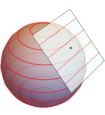
I previously wrote about a connection for a spherically symmetric vector field. This has been a good learning experience about connections other than Levi-Civita. Many of us completed general relativity courses in which the curvature quantities were merely formulae with no intuitive understanding. However questions from mathematicians like: “Which connection are you using?” prompted me to learn more. (At least I have never been asked which differential structure I am using, nor which point-set topology, which is fortunate for all involved. 🙂 ) There are various physically-motivated connections defined in research paper research paper (arXiv) §2. I intend to apply this to the rotating disc, and to an observer field in Schwarzschild spacetime. Also, I accidentally came across Rothman+ 2001 about parallel transport in Schwarzschild spacetime, with numerous followup papers by various authors. All of this struck me again with a sense of fascination about curvature: how rich and deep it is.

🡐 Spherical symmetry connection | Curvature | ⸻ 🠦

Local Lorentz boost in coordinate-independent notation

Difficulty: ★★★☆☆ undergraduate

The Lorentz boost between two reference frames can be expressed as a (1,1)-tensor $\boldsymbol\Lambda$ , interpreted as an operator on vectors. Here we re-express this well known fact using a general, index-free, coordinate-independent, 4-vector notation, which is valid locally in curved spacetime.

Recall the prototypical Lorentz boost on Minkowski spacetime:

$\Lambda^\mu_{\hphantom\mu\nu} = \begin{pmatrix} \gamma & -\beta\gamma & 0 & 0 \\ -\beta\gamma & \gamma & 0 & 0 \\ 0 & 0 & 1 & 0 \\ 0 & 0 & 0 & 1 \end{pmatrix}.$

This is a boost in the $x$ -direction by speed $\beta$ or Lorentz factor $\gamma = (1-\beta^2)^{-1/2}$ . It maps an arbitrary vector $X^\mu$ to $\Lambda^\mu_{\hphantom\mu\nu}X^\nu$ . Numerous authors generalise to arbitrary boost directions, such as Møller book §18; MTW book §2.9; or Tsamparlis book §1.7. This typically involves separate transformations of time and 3-dimensional space: $t' = \gamma(t - \vec n\cdot\vec r)$ and $\vec r' = \vec r + (\frac{\gamma-1}{\beta^2}\vec r\cdot\vec n - \gamma t)\vec n$ . The arrows signify 3-dimensional vectors, $\vec r$ is the position in 3-space, and $\vec n$ is the relative 3-velocity. The space part uses beautiful, coordinate-independent vector language. However the time part requires privileged coordinates adapted to the observers. We will derive a 4-vector analogue.

Consider two 4-velocity vectors $\mathbf u$ and $\mathbf n$ (located at the same point, if in curved spacetime). They are related by the Lorentz boost:

$\mathbf n = \gamma(\mathbf u+\beta\hat{\vec{\mathbf n}}) = \gamma(\mathbf u+\vec{\mathbf n}),$

where $\gamma = -\langle\mathbf u,\mathbf n\rangle$ , the unit vector $\hat{\vec{\mathbf n}}$ points in the boost direction, and $\vec{\mathbf n} = \beta\hat{\vec{\mathbf n}}$ is the relative velocity. This is the 4-vector analogue of the familiar coordinate boost $t' = \gamma(t-\beta x)$ . Combined with the space boost given shortly, this forms a local Lorentz transformation. While the plus sign makes the above appear an inverse boost, this is only because vectors (as whole entities) transform inversely to coordinates. Rearranging:

$\vec{\mathbf n} = \gamma^{-1}\mathbf n - \mathbf u.$

This is the relative velocity of the observer $\mathbf n$ as determined in $\mathbf u$ ’s frame, as explained previously. It is equivalent to the $\vec n$ introduced in the 3-dimensional spatial transformation, except now treated as a 4-vector. It is orthogonal to $\mathbf u$ , with length $\beta$ . Conversely, the relative velocity of $\mathbf u$ as determined in $\mathbf n$ ’s frame is $\vec{\mathbf u} = \gamma^{-1}\mathbf u - \mathbf n$ . Now, the vector analogue of the usual boosted spatial coordinate $x' = \gamma(x-\beta t)$ is $\gamma(\hat{\vec{\mathbf n}}+\beta\mathbf u)$ . After multiplying by $\beta$ :

$\vec{\mathbf n} \mapsto \gamma(\vec{\mathbf n} + \beta^2\mathbf u) = \mathbf n - \gamma^{-1}\mathbf u = -\vec{\mathbf u}.$

Hence the relative velocity vectors are boosted into one-another, aside from a minus sign (Jantzen+ 1992 research paper (arXiv) §4). This generalises the Newtonian result $\vec n = -\vec u$ . So we have the boost’s action on the orthogonal vectors $\mathbf u$ and $\vec{\mathbf n}$ , plus it is the identity on the 2-dimensional spatial plane orthogonal to both, hence:

$\begin{aligned} \Lambda^\mu_{\hphantom\mu\nu} &= (g^\mu_{\hphantom\mu\nu} + u^\mu u_\nu -\beta^{-2}\vec n^\mu \vec n_\nu) - n^\mu u_\nu -\beta^{-2}\vec u^\mu \vec n_\nu \\ &= g^\mu_{\hphantom\mu\nu} + (u^\mu-n^\mu)u_\nu + \frac{\gamma}{\gamma+1}(u^\mu + n^\mu)\vec n_\nu, \end{aligned}$

using $\vec{\mathbf u}+\vec{\mathbf n} = -(1-\gamma^{-1})(\mathbf u+\mathbf n)$ and $(\gamma-1)/\beta^2\gamma = \gamma/(\gamma+1)$ . It is a good exercise to check the contractions with $u^\nu$ , $\vec n^\nu$ , or any $X^\nu$ orthogonal to both. In index-free notation,

$\boldsymbol\Lambda = \mathbf g^{\sharp\flat} + (\mathbf u-\mathbf n)\otimes\mathbf u^\flat +\frac{\gamma}{\gamma+1}(\mathbf u+\mathbf n)\otimes\vec{\mathbf n}^\flat.$

The “flat” symbol just means: lower an index. Equivalently, in terms of the initial observer and boost velocity alone:

$\boldsymbol\Lambda = \mathbf g^{\sharp\flat} + \big((1-\gamma)\mathbf u - \gamma\vec{\mathbf n})\otimes\mathbf u^\flat + \big(\gamma\mathbf u + \frac{\gamma^2}{\gamma+1}\vec{\mathbf n}\big)\otimes\vec{\mathbf n}^\flat,$

in which case the relative speed may be obtained from $\beta^2 = \langle\vec{\mathbf n},\vec{\mathbf n}\rangle$ . This is equivalent to MTW’s Exercise 2.7 which uses Cartesian coordinates, after adjusting various minus signs because I use vectors not vector components. In terms of the 4-velocities alone, we have the curiously symmetric expression:

$\boldsymbol\Lambda = \mathbf g^{\sharp\flat} + \frac{1}{\gamma+1} (\mathbf u+\mathbf n)\otimes(\mathbf u+\mathbf n)^\flat - 2\mathbf n\otimes\mathbf u^\flat.$

Formulae are useful machines, allowing you to blithely turn the handle to crank out a result. This contrasts with my usual emphasis on conceptual understanding, and drawing a picture (at least mentally). However Lorentz boosts have many counter-intuitive or seemingly paradoxical effects. It is easier to make a mistake if you reason from first-principles alone. Of course the algebra does originate from careful thinking about foundations, and having multiple approaches is a check of consistency.

Boosts are paramount for comparing physical quantities between frames. Some textbooks present the general Lorentz boost in Minkowski spacetime with Cartesian coordinates. Our abstract vector formulation allows direct application to local boosts in arbitrary spacetime, such as Kerr or FLRW, in any coordinate system. I don’t remember seeing the formulae here in the literature, but someone should have done it somewhere. The Jantzen+ paper was an inspiration, and the same authors define various further quantities (projections, in fact) in Bini+ 1995 research paper (astronomy) .

🡐 relative velocity | relative kinematics | ⸻ 🠦

Spatial gradient examples

Difficulty: ★★★☆☆ undergraduate

Last time we discussed the “spatial gradient” or “3-gradient”, and here we follow up with two examples. Recall from before that a scalar field $\Phi$ has gradient $d\Phi$ , and the part of this which is orthogonal to an observer 4-velocity $\mathbf u$ is, as a vector:

$^{(3)}(d\Phi)^\sharp := (d\Phi)^\sharp + \langle d\Phi,\mathbf u\rangle \mathbf u.$

This direction has the greatest increase of $\Phi$ , for any vector in $\mathbf u$ ’s 3-space (that is, orthogonal to $\mathbf u$ ), per length of the vector.

As an example, suppose the 4-gradient vector $(d\Phi)^\sharp$ is a null, future-pointing vector. It can be decomposed $E(\mathbf u+\boldsymbol\xi)$ , where $E := -\langle d\Phi,\mathbf u\rangle$ , and $\boldsymbol\xi$ is a unit spatial vector orthogonal to $\mathbf u$ . Physically, this gradient may be interpreted as a null wave or photon, which the observer determines to have energy (or related quantity, such as frequency) $E$ , and to move in the spatial direction $\boldsymbol\xi$ . The 3-gradient vector is $E\boldsymbol\xi$ , hence the direction of relative velocity also has the steepest increase of $\Phi$ , within the observer’s 3-space.

Suppose now $(d\Phi)^\sharp$ is a unit, timelike, future-pointing vector, so that we may interpret it as the 4-velocity $\mathbf v$ of a second observer. Then $^{(3)}(d\Phi)^\sharp = \mathbf v - \gamma\mathbf u$ , where $\gamma = - \langle\mathbf u,\mathbf v\rangle$ is the Lorentz factor between the pair. But we also have the “relative velocity” decomposition $\mathbf v = \gamma(\mathbf u + \mathbf V)$ , where $\mathbf V$ is the relative velocity of $\mathbf v$ as determined in $\mathbf u$ ’s frame, as I discussed previously. Combining these, $^{(3)}(d\Phi)^\sharp = \gamma\mathbf V$ . 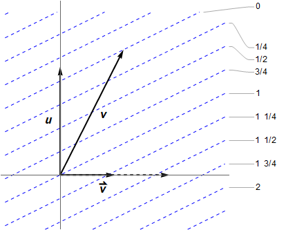Hence within the observer’s 3-space, $\Phi$ again increases most sharply in the direction of the relative velocity.

Spacetime diagram, from the observer $\mathbf u$ ‘s perspective. The timelike 1-form $d\Phi \equiv \mathbf v^\flat$ is suggested by dotted blue lines, given at intervals of 1/4 for more resolution. These are orthogonal to the vector $\mathbf v$ , in the Lorentzian sense.

The figure shows the single tangent space — think of this as the linearisation of what is happening locally over the manifold itself. The hyperplanes are numbered by $\Phi$ , where only the differences between them are relevant, as an overall constant was not specified. Observe $\mathbf v$ crosses four of them, spanning an interval $\Delta\Phi = \langle d\Phi,\mathbf v\rangle = -1$ , so $\Phi$ is the negative of $\mathbf v$ ’s proper time; see a previous post for more background. In both our examples, the scalar decreases towards the future (or can vanish in the null case), even though the gradient vectors are future-pointing. That is, the gradient vectors actually point “down” the slope! This quirk is due to our −+++ metric signature, and would apply to spacelike gradients if +−−− were used instead. This really hurt my brain, until I drew the diagram. 🙁

To construct it, consider the action of $d\Phi$ on the axes. The horizontal axis is the relative velocity direction, with unit vector $\hat{\mathbf V} := \mathbf V/\beta$ . One can show $\langle d\Phi,\hat{\mathbf V}\rangle = \beta\gamma$ . Also $\langle d\Phi,\mathbf u\rangle = -\gamma$ , but I find it easier to think of: $\langle d\Phi,-\mathbf u\rangle = \gamma$ . These give the number of hyperplanes crossed by the unit axes vectors, then you can literally “connect the dots” since the 1-form is linear. In the figure $\beta = 1/2$ , so $\gamma \approx 1.15$ . (As for the 3-gradient, it vanishes in the $\mathbf u$ direction, hence $\mathbf u$ must cross no contours of $^{(3)}d\Phi$ . It would be drawn as vertical lines, with corresponding vector pointing to the right.)

Most of our discussion applies to arbitrary 1-forms, not just gradients which are termed exact 1-forms. I derived the work here independently, but the literature contains some similar material. It turns out Jantzen, Carini & Bini 1992 research paper (arXiv) §2 explicitly define the “spatial gradient”, as they most appropriately call it. A few textbooks discuss scalar waves, for which the 3-gradient vector is the wave 3-vector, which is orthogonal to the wavefronts within a given frame, as discussed shortly.

Spatial gradient of a scalar

Difficulty: ★★★☆☆ undergraduate

Suppose you have a scalar field $\Phi$ , and at a given point in spacetime: a 4-velocity vector interpreted as an “observer”. In which direction does $\Phi$ increase most steeply, when restricted to the observer’s local 3-dimensional space?

Last time I reviewed the gradient 1-form or covector $d\Phi$ , and its associated gradient vector $(d\Phi)^\sharp$ obtained by raising the index as usual. The gradient vector has been described as the direction of greatest increase in $\Phi$ per unit length (Schutz 2009 book §3.3). However this is only guaranteed when the metric is positive definite, meaning a Riemannian manifold, rather than a Lorentzian manifold as used to model spacetime.

The observer’s 4-velocity splits vectors and 1-forms into purely “time” parts parallel to $\mathbf u$ , and purely “space” parts orthogonal to it. (Intuitively, it may help to think of a basis $\{\mathbf e_\alpha\}$ adapted to the observer, meaning $\mathbf e_0 := \mathbf u$ , and the $\mathbf e_i$ vectors are orthogonal to $\mathbf u$ , where $i = 1,2,3$ . Then a purely spatial vector is spanned by the $\mathbf e_i$ . Since vectors and covectors are linear, we need only specify their values on a basis set.)

Consider the tangent space at the specified point. Imagine working within the observer’s local 3-space, by which I mean the 3-dimensional subspace consisting of vectors orthogonal to $\mathbf u$ . Label the gradient as restricted to this subspace by $^{(3)}d\Phi$ . On the subspace the metric has Riemannian signature, hence the corresponding vector $^{(3)}(d\Phi)^\sharp$ is the direction of steepest increase. We can mimic this mathematically by staying in 4 dimensions, but setting the “time” part to zero:

$^{(3)}d\Phi := d\Phi + \langle d\Phi,\mathbf u\rangle \mathbf u^\flat.$

This is a 4-dimensional object, but I reuse the notation “ $^{(3)}$ ” to imply it vanishes in the observer’s time direction. This “3-gradient” is the projection of $d\Phi$ orthogonal to $\mathbf u^\flat$ . The angle brackets signify contraction of the 1-form and vector, and the “flat” symbol denotes the 1-form obtained from $\mathbf u$ by “lowering the index” using the metric. The vector 3-gradient is:

$^{(3)}(d\Phi)^\sharp = (d\Phi)^\sharp + \langle d\Phi,\mathbf u\rangle \mathbf u.$

This follows from “raising the index” using the inverse metric $g^{\mu\nu}$ as usual. Note that on the subspace, the inverse metric coincides with the inverse 3-metric which has components $(g_{ij})^{-1}$ , for $i,j=1,2,3$ . Equivalently, one can apply the spatial projector $g^{\mu\nu}+u^\mu u^\nu$ to either $d\Phi$ or $^{(3)}d\Phi$ , with the same result. This projector agrees with the inverse metric on the 3-space, and is zero on purely timelike covectors. Either way, the essential part of the process is to remove the “time” component of the gradient. I will give examples in the following post.

Gradient of a scalar

Difficulty: ★★★☆☆ undergraduate

Suppose a scalar field $\Phi$ is defined on some region of spacetime. Its gradient $d\Phi\equiv \nabla\Phi$ expresses the change in $\Phi$ (that is, its derivative) in each direction. In a coordinate system, it has components:

$\nabla_\mu\Phi = (d\Phi)_\mu = \Phi_{,\mu} := \frac{\partial\Phi}{\partial x^\mu}.$

$d\Phi$ is a 1-form or covector. [Recall a 1-form is just a (0,1)-tensor. Schutz 2009 book also uses the term dual vector, though I find this can lead to clumsy wording, such as the hypothetical phrase: “the vector [which is] dual to a dual vector”. Traditionally the term covariant vector has been used, meaning its components transform “covariantly” with a change of basis. 1-forms are a rigorous version of differentials, superceding the older idea of infinitesimals but using similar notation (Schutz 1980 book §2.19; Spivak vol. 1 book §4).] Above, “ $d$ ” is called the exterior derivative, and $\nabla$ is the covariant derivative, but when acting on a scalar these coincide. Recall a 1-form accepts a vector and returns a number. In this case, the vector is the direction of differentiation, and the output is the derivative of $\Phi$ in that direction (where the vector’s magnitude matters also).

The 1-form $d\Phi$ may be visualised as a set of hypersurfaces or level sets $\Phi = \textrm{const}$ , on the manifold (MTW book §2.5–2.7, Box 4.4; Schutz 2009 §3.3). Ideally these could be spaced at intervals $\Delta\Phi = 1$ . Given some vector $\mathbf Y$ , the contraction:

$d\Phi(\mathbf Y) \equiv \langle d\Phi,\mathbf Y\rangle = Y^\mu\frac{\partial\Phi}{\partial x^\mu}$

is visualised as the number of hypersurfaces the vector pierces, or “bongs of [a] bell” in MTW’s colourful terminology. Technically however, vectors and 1-forms exist in the (co-)tangent spaces, not extended along the manifold. At any given point, $d\Phi$ is the linear approximation to $\Phi$ , ignoring the constant term (MTW §2.6). Hence $d\Phi$ is more accurately visualised as hyperplanes within the tangent space there. The diagram below shows both artistic choices. Note in two dimensions, hypersurfaces and hyperplanes are just curves and straight lines, respectively.

sphere with dtheta field — A 2-sphere with visualisations of the 1-form field $d\theta$ , both over the entire manifold and within a single tangent space. The spacing is $\Delta\theta = \pi/10$ .

The gradient vector is the dual to $d\Phi$ , with components obtained by raising the index in the usual way: $g^{\mu\nu}(d\Phi)_\nu$ . This may be elegantly written $(d\Phi)^\sharp$ , where the “sharp” symbol is part of the “musical isomorphism” notation. While the gradient is usually first encountered as a vector, it is most naturally a 1-form, as this does not require a metric (MTW §9.4). As Schutz 2009 §3.3 explains:

…we in general cannot call a gradient a vector. We would like to identify the vector gradient as that vector pointing ‘up’ the slope, i.e. in such a way that it crosses the greatest number of contours per unit length. The key phrase is ‘per unit length’. If there is a metric, a measure of distance in the space, then a vector can be associated with a gradient. But the metric must intervene here in order to produce a vector. Geometrically, on its own, the gradient is a one-form.

But if one does not know how to compare the lengths of vectors that point in different directions, one cannot define a direction of steepest ascent…

The last line is from Schutz 1980 §2.19, where the discussion is similar. These textbooks give a superb introductory account of 1-forms, however the steepness comments are only valid for a Riemannian metric, with positive-definite signature. Consider Minkowski spacetime with coordinates $(t,x,y,z)$ . By linearity, we need only consider unit vectors. The 1-form $dx$ has components $(0,1,0,0)$ , with $(dx)^\sharp$ just $\partial_x$ . These contract to give unity. If we restrict to vectors spanned by $\partial_x$ , $\partial_y$ and $\partial_z$ , Schutz’ steepness comments apply. However $\pm(\beta\gamma,\gamma,0,0)$ is also a unit spacelike vector, where $\gamma = (1-\beta^2)^{-1/2}$ , but combines with $dx$ to give $\pm\gamma$ , hence crosses more intervals $x = \textrm{const}$ than the gradient vector does. Similarly for $dt$ , the contraction with $(dt)^\sharp = -\partial_t$ returns $-1$ , but with the unit timelike vector $\pm(\gamma,\beta\gamma,0,0)$ yields $\pm\gamma$ . Hence for a timelike 1-form, its gradient vector crosses the least contours (taking the absolute value) per unit length, compared to other timelike vectors only. For a null 1-form, its gradient vector lies along the hyperplanes, so crosses zero of them (MTW Figure 2.7)!

Instead, we are left with saying the gradient vector is orthogonal to all vectors $\mathbf Y$ on which the 1-form vanishes: $\langle (d\Phi)^\sharp,\mathbf Y\rangle = 0$ whenever $\langle d\Phi,\mathbf Y\rangle = 0$ . The angle brackets mean contraction using the metric, with indices appropriately raised or lowered. Another property is the gradient vector’s squared-norm equals the 1-form’s squared-norm, which also matches the number of contours crossed:

$\langle (d\Phi)^\sharp,(d\Phi)^\sharp\rangle = \langle d\Phi,d\Phi\rangle = \langle d\Phi,(d\Phi)^\sharp\rangle.$

The above statements are basically tautologies, but they help clarify what metric duality means. Incidentally, not all 1-forms arise as the “ $d$ ” of a scalar, but only those termed exact (Wald book §B1). Most of this post applies also to arbitrary 1-forms $\boldsymbol\alpha$ , for which the hyperplanes are spanned by vectors satisfying $\langle\boldsymbol\alpha,\mathbf Y\rangle = 0$ . For many creative illustrations see MTW, including their “honeycomb” and “egg crate” analogies for 2-forms and 3-forms, and their Figure 4.5 for the 2-form $d\theta\wedge d\phi$ . Finally, I previously reviewed contractions like $d\Phi(\mathbf u) = d\Phi/d\tau$ , which give the rate of change of the scalar by proper time along a worldline.