The discovery of spinors is most often credited to quantum physicists in the 1920s, and to Élie Cartan in the prior decade for an abstract mathematical approach. But it turns out the legendary mathematician Leonhard Euler discovered certain algebraic properties for the usual (2-component, Pauli) spinors, back in the 1700s! He gave a parametrisation for rotations in 3D, using essentially what were later known as Cayley-Klein parameters. There was not even the insight that each set of parameter values forms an interesting object in its own right. But we can recognise one key conceptual aspect of spinors in this accidental discovery: the association with rotations.
In 1771, Euler published a paper on orthogonal transformations, whose title translates to: “An algebraic problem that is notable for some quite extraordinary relations”. Euler scholars index it as “E407”, and the Latin original  is available from the Euler Archive website. I found an English translation online, which also transcribes the original language.
Euler commences with the aim to find “nine numbers… arranged… in a square” which satisfy certain conditions. In modern notation this is a matrix M say, satisfying  , which describes an orthogonal matrix. While admittedly the paper is mostly abstract algebra, he is also motivated by geometry. In §3 he mentions that the equation for a surface is “transformed” under a change of [Cartesian] coordinates, including the case where the coordinate origins coincide. We recognise this (today, at least) as a rotation, possibly combined with a reflection. Euler also mentions “angles” (§4 and later), which is clearly geometric language.
He goes on to analyse orthogonal transformations in various dimensions. [I was impressed with the description of rotations about n(n – 1)/2 planes, in n dimensions, because I only first learned this in the technical context of higher-dimensional rotating black holes. It is only in 3D that rotations are specified by axis vectors.] Then near the end of the paper, Euler seeks orthogonal matrices containing only rational entries, a “Diophantine” problem. Recall rotation matrices typically contain many trigonometric terms like sin(θ) and cos(θ), which are irrational numbers for most values of the parameter θ. But using some free parameters “p, q, r, s”, Euler presents:
![\[\begin{tabular}{|c|c|c|}\hline $\frac{p^2+q^2+r^2+s^2}{u}$ & $\frac{2(qr+ps)}{u}$ & $\frac{2(qs-pr)}{u}$ \\ \hline $\frac{2(qr-ps)}{u}$ & $\frac{p^2-q^2+r^2-s^2}{u}$ & $\frac{2(pq+rs)}{u}$ \\ \hline $\frac{2(qs+pr)}{u}$ & $\frac{2(rs-pq)}{u}$ & $\frac{p^2-q^2-r^2+s^2}{u}$ \\ \hline\end{tabular},\]](http://cmaclaurin.com/cosmos/wp-content/ql-cache/quicklatex.com-8a820b1a5889a514cf73584ad468f584_l3.png "Rendered by QuickLaTeX.com")
where  . (I have copied the style which Euler uses in some subsequent examples.) By choosing rational values of the parameters, the matrix entries will also be rational, however this is not our concern here. The matrix has determinant +1, so we know it represents a rotation. It turns out the parameters form the components of a spinor!!
  are the real components of a normalised spinor. We allow all real values, but will ignore some trivial cases. One aspect of spinors is clear from inspection: in the matrix the parameters occur only in pairs, hence the sets of values and
  give rise to the same rotation matrix. (Those familiar with spinors will recall the spin group is the “double cover” of the rotation group.)
The standard approach is to combine the parameters into two complex numbers. But in the geometric algebra (or Clifford algebra) interpretation, a spinor is a rotation of sorts, or we might say a “half-rotation”. It is about the following plane:
![\[q\hat{\mathbf y}\wedge\hat{\mathbf z} + r\hat{\mathbf z}\wedge\hat{\mathbf x} + s\hat{\mathbf x}\wedge\hat{\mathbf y}.\]](http://cmaclaurin.com/cosmos/wp-content/ql-cache/quicklatex.com-46fe75d65665b9ede3e4bcd9bc9e579a_l3.png "Rendered by QuickLaTeX.com")
(For those who haven’t seen the wedge product nor bivectors, you can visualise  for example, as the parallelogram or plane spanned by those vectors. It also has a magnitude and handedness/orientation.) The sum is itself a plane, because we are in 3D. Dividing by
  gives a unit bivector. For the spinor, the angle of rotation θ/2 say, is given by (c.f. Doran & Lasenby 2003
  §2.7.1):
![\[\cos(\theta/2) = p/\sqrt{u},\qquad \sin(\theta/2) = \sqrt{(q^2+r^2+s^2)/u}.\]](http://cmaclaurin.com/cosmos/wp-content/ql-cache/quicklatex.com-3129e321d8198223313e27e17b0297f0_l3.png "Rendered by QuickLaTeX.com")
This determines θ/2 to within a range of 2π (if we include also the orientation of the plane). In contrast, the matrix given earlier effects a rotation by θ — twice the angle — about the same plane. This is because geometric algebra formulates rotations using two copies of the spinor. The matrix loses information about the sign of the spinor, and hence also any distinction between one or two full revolutions.
Euler extends the challenge of finding orthogonal matrices with rational entries to 4D. In §34 he parametrises matrices using “eight numbers at will a, b, c, d, p, q, r, s”. However the determinant of this matrix is -1, so it is not a rotation, and the parameters cannot form a spinor. Two of its eigenvalues are -1 and +1. Now the eigenvectors corresponding to distinct eigenvalues are orthogonal (a property most familiar for symmetric matrices, but it holds for orthogonal matrices also). It follows the matrix causes reflection along one axis, fixes an orthogonal axis, and rotates about the remaining plane. So it does not “include every possible solution” (§36). But I guess the parameters might form a subgroup of the Pin(4) group, the double cover of the 4-dimensional orthogonal group O(4).
Euler provides another 4×4 orthogonal matrix satisfying additional properties, in §36. This one has determinant +1, hence represents a rotation. It would appear no eigenvalues are +1 in general, so it may represent an arbitrary rotation. I guess the parameters  , where I label by u the quantity
  mentioned by Euler, might form spinors of 4D space (not 3+1-dimensional spacetime). If so, these are members of Spin(4), the double cover of the 4D rotation group SO(4).
Euler was certainly unaware of his implicit discovery of spinors. His motive was to represent rotations using rational numbers, asserting these are “most suitable for use” (§11). Probably more significant today is that rotations are described by rational functions of spinor components. But the fact spinors would be rediscovered repeatedly in different applications suggests there is something very natural or Platonic about them. Euler says his 4D “solution deserves the more attention”, and that with a general procedure for this and higher dimensions, “Algebra… would be seen to grow very much.” (§36) He could not have anticipated how deserving of attention spinors are, nor their importance in algebra and elsewhere!


 , or
, or  for an arbitrary frame. In particular, each cobasis element is orthogonal to the “other” 3 vectors. But we can take the duals
  , which are vectors but obey the same orthogonality relations, via the metric scalar product:
  . (By relating to the standard approach I may have made things look complicated, but this should be visualised as simply finding new vectors orthogonal to existing vectors.) (On a separate note, “dual” here means
  (Doran & Lasenby 2003
 ![\[P(I,N|i\textrm{ died on }n) = a_{I-i,N-n}.\]](http://cmaclaurin.com/cosmos/wp-content/ql-cache/quicklatex.com-1ab856289d606cb0c4d6dd4c6f2308d8_l3.png "Rendered by QuickLaTeX.com")
 is the chance player i′ is alive on step n′ (given no information nor conditions). We labelled as
  the chance they died on step n′ specifically, so analogously:
![\[P(I\textrm{ dies on }N|i\textrm{ died on }n) = b_{I-i,N-n}.\]](http://cmaclaurin.com/cosmos/wp-content/ql-cache/quicklatex.com-dd3fdc90b7b92118408f0173d76a8462_l3.png "Rendered by QuickLaTeX.com")
 , which in our case is:
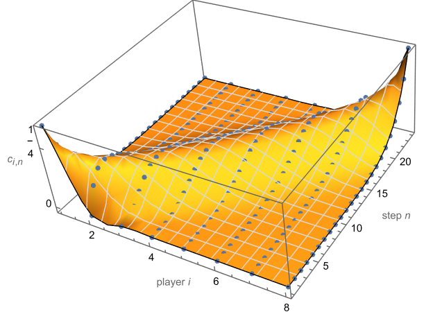
![\[\begin{aligned}c_{i,n} &:= P(i\textrm{ died on }n|I\textrm{ dies on }N) \\ &= \frac{b_{I-i,N-n}b_{i,n}}{b_{I,N}} \\ &= \frac{\binom{N-n-1}{I-i-1}\binom{n-1}{i-1}}{\binom{N-1}{I-1}}.\end{aligned}\]](http://cmaclaurin.com/cosmos/wp-content/ql-cache/quicklatex.com-0fdbd6c888443c4ffb02f41beb3ab8bb_l3.png "Rendered by QuickLaTeX.com")
 computer algebra returns a hypergeometric function times two binomial coefficients, which appears to simplify to 1 (for integer parameters) as expected, since player i must die somewhere. On any given column
  which is independent of n, meaning each step has equal chance that some player will die there. In particular the first entry itself takes this value:
  .
. ; our general formula does not apply for n = N. If we are told where the second player I = 2 died, then player i = 1 has an equal chance 1/(N – 1) of dying on any earlier step. Also from the definition it is clear:
![\[c_{i,n} \equiv c_{I-i,N-n},\]](http://cmaclaurin.com/cosmos/wp-content/ql-cache/quicklatex.com-c4a6b15f93b0f58c1ed010993677e8e8_l3.png "Rendered by QuickLaTeX.com")
![\[\begin{aligned}\frac{c_{i-1,n}}{c_{i,n}} &= \frac{(i-1)(N-I-n+i)}{(I-i)(n-i+1)}, \\ \frac{c_{i,n-1}}{c_{i,n}} &= \frac{(N-n)(n-i)}{(n-1)(N-I-n+i+1)}.\end{aligned}\]](http://cmaclaurin.com/cosmos/wp-content/ql-cache/quicklatex.com-23abcecbb3de8058f61c88bc262b341a_l3.png "Rendered by QuickLaTeX.com")
![\[c_{i,n} \equiv \frac{i\binom{N-I}{n-i}\binom{I-1}{i}}{n\binom{N-1}{n}}.\]](http://cmaclaurin.com/cosmos/wp-content/ql-cache/quicklatex.com-8c9a9276cb95c0054bd27bee7f5646bd_l3.png "Rendered by QuickLaTeX.com")
![\[-\frac{\Big(i-\frac{N+nI-I-2n}{N-2}\Big)^2}{(n-1)(N-n-1)/2(N-2)}.\]](http://cmaclaurin.com/cosmos/wp-content/ql-cache/quicklatex.com-243c5e79f2f06bb5cc95404001c8b671_l3.png "Rendered by QuickLaTeX.com")
 ,
,  ,
,  , and
, and  . The centre is
  . One option for the height of the gaussians — when looking for a simple expression — is to use the sums 1 and (I – 1)/(N – 1) determined before. Recall for a normalised gaussian, the height
  is inversely proportional to the standard deviation.
 , where we also substitute
  and
and  . As another possible scenario to analyse, we might be informed that player I is alive on step N. Then we would not know how far they progressed, just that it was at least that far. Or, we might be told player I died on or before step N.
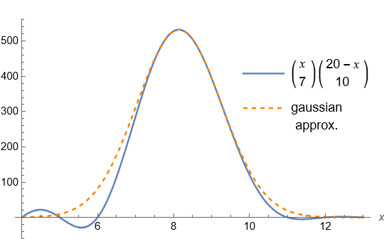
![\[f(x) := \binom{x}{a}\binom{X-x}{b}.\]](http://cmaclaurin.com/cosmos/wp-content/ql-cache/quicklatex.com-1c69da7feadf7542bab4557bbee83d88_l3.png "Rendered by QuickLaTeX.com")
 , and this is extended beyond integer values by replacing each factorial with a Gamma function. Note the independent variable x appears in the upper entries of the binomial coefficients. Curiously, from inspection f is well-approximated by a gaussian curve. To gain some insight, for integer values of the parameters f is the polynomial:
![\[(a! b!)^{-1}x(x-1)\cdots(x-a+1)\cdot(X-b+1-x)\cdots(X-x).\]](http://cmaclaurin.com/cosmos/wp-content/ql-cache/quicklatex.com-b20d4e7b8bc3483c861c39a29b20c96f_l3.png "Rendered by QuickLaTeX.com")
 , where the H’s are called harmonic numbers. There may not exist any simple explicit expression for the turning points. Instead, the ratio of nearby points is comparatively simple:
![\[\frac{f(x-1/2)}{f(x+1/2)} = \frac{(x-a+1/2)(X+1/2-x)}{(x+1/2)(X-b+1/2-x)},\]](http://cmaclaurin.com/cosmos/wp-content/ql-cache/quicklatex.com-57dd3410e47df89c49bba1c3de59ad63_l3.png "Rendered by QuickLaTeX.com")
![\[x_0 := \frac{2aX+a-b}{2(a+b)}.\]](http://cmaclaurin.com/cosmos/wp-content/ql-cache/quicklatex.com-e1e66503da60cec1c6fbc07436179f21_l3.png "Rendered by QuickLaTeX.com")
 . We set the height
  . Only the width remains to be determined. The gaussian’s second derivative evaluated at its centre point is
  . On the other hand:
![\[f''(x) = f'(x)^2/f(x) - (H_x^{(2)}-H_{x-a}^{(2)}+H_{X-x}^{(2)}-H_{X-b-x}^{(2)})f(x),\]](http://cmaclaurin.com/cosmos/wp-content/ql-cache/quicklatex.com-7ad361f0313f7ef917aaff2215d6ae89_l3.png "Rendered by QuickLaTeX.com")
 yields the variance parameter
  :
:![\[\sigma^{-2} := H_{x_0}^{(2)}-H_{x_0-a}^{(2)}+H_{X-x_0}^{(2)}-H_{X-b-x_0}^{(2)},\]](http://cmaclaurin.com/cosmos/wp-content/ql-cache/quicklatex.com-ead1aeb4d9408b154175be6911c0ad75_l3.png "Rendered by QuickLaTeX.com")
 . (At large values the series
  may give insight into the above.) But alternatively, we can approximate the second derivative using elementary operations. By sampling the function at
  ,
,  say, a “finite differences” approach gives approximate derivatives. We can use the simple ratio formula obtained earlier to reduce the sampling to one or two points only, which might gain some insight along the way (though I currently wonder if this is a dead end…).
 , which becomes:
![\[\frac{2C(a+b)^3}{(2aX+a-b)(2bX-2b^2-2ab+a+3b)},\]](http://cmaclaurin.com/cosmos/wp-content/ql-cache/quicklatex.com-246c69ac64e3e9b91c1b8ecff72861e3_l3.png "Rendered by QuickLaTeX.com")
 in terms of C. Similarly it turns out
  is the negative of the above expression, but with a and b interchanged. Then a second derivative is:
  , but the combined expression does not simplify further so I won’t write it out. The last step is to set
  , which is different to the earlier choice.
 , which may be expressed in terms of another sampled point
  . Similarly
  . The estimate for the second derivative follows, then later:
![\[\hat\sigma^2 := \frac{-2C(aX-b)(bX+a+2b)(bX-b^2-ab+a+2b)(aX-a^2-ab-b)}{E(a+b)^6}.\]](http://cmaclaurin.com/cosmos/wp-content/ql-cache/quicklatex.com-26104a688f522ab5ac0d8b4cead8903b_l3.png "Rendered by QuickLaTeX.com")
 and
and  instead leads to the same result.
![\[x^A(X-x)^B,\]](http://cmaclaurin.com/cosmos/wp-content/ql-cache/quicklatex.com-b903e544044457f900ec1394a27ba646_l3.png "Rendered by QuickLaTeX.com")
 .
. ![x \in [0,X]](http://cmaclaurin.com/cosmos/wp-content/ql-cache/quicklatex.com-a0e5301bb389911858235676d9461dd2_l3.png "Rendered by QuickLaTeX.com") .
.
 , and for each non-integer exponent the tail on one side becomes imaginary.
![\[\tilde x := \frac{X}{1+B/A},\]](http://cmaclaurin.com/cosmos/wp-content/ql-cache/quicklatex.com-63503dd0564d1a52ac96d3a1640448a1_l3.png "Rendered by QuickLaTeX.com")
![\[A^A B^B \Big(\frac{X}{A+B}\Big)^{A+B} \equiv (B/A)^B \tilde x^{A+B}.\]](http://cmaclaurin.com/cosmos/wp-content/ql-cache/quicklatex.com-aeebf08eeae9091455a082f773ef460e_l3.png "Rendered by QuickLaTeX.com")
 . This has centre D which we equate with
  , and maximum height C which we set to the above expression. We can fix the final parameter, the standard deviation, by matching the second derivatives at the turning point. Hence the variance is:
![\[\sigma^2 = \frac{AB}{(A+B)^3}X^2 \equiv \frac{B}{A^2X}\tilde x^3.\]](http://cmaclaurin.com/cosmos/wp-content/ql-cache/quicklatex.com-a9b3e559a77aa85b702f021ab451ce4b_l3.png "Rendered by QuickLaTeX.com")
![\[\boxed{(B/A)^B \tilde x^{A+B} \operatorname{exp}\Big( -\frac{(x-\tilde x)^2}{2B\tilde x^3/A^2X} \Big).}\]](http://cmaclaurin.com/cosmos/wp-content/ql-cache/quicklatex.com-231edb19ae54a811f95077fe10c1f232_l3.png "Rendered by QuickLaTeX.com")
![\[\int_0^X x^A(X-x)^Bdx = \frac{X^{A+B+1}}{(A+B+1)\binom{A+B}{A}}.\]](http://cmaclaurin.com/cosmos/wp-content/ql-cache/quicklatex.com-62f1b0ae17cb0881a5e0f7f01c59ce05_l3.png "Rendered by QuickLaTeX.com")
 , which is extended to non-integer values by replacing the factorials with Gamma functions. We could then apply Stirling’s approximation
  to each factorial, to obtain:
![\[\int\cdots \approx \frac{\sqrt{2\pi(A+B)}}{A+B+1}(B/A)^{B+1/2}\tilde x^{A+B+1},\]](http://cmaclaurin.com/cosmos/wp-content/ql-cache/quicklatex.com-8e45ac6bded4d3733a9f18fd0fe8b6d3_l3.png "Rendered by QuickLaTeX.com")
![\[\int_{-\infty}^\infty \operatorname{exp}\cdots = \sqrt\frac{2\pi}{A+B}(B/A)^{B+1/2}\tilde x^{A+B+1}.\]](http://cmaclaurin.com/cosmos/wp-content/ql-cache/quicklatex.com-6a1d3bd57315c5c72453e2f129c53372_l3.png "Rendered by QuickLaTeX.com")
 .
.![\[P(i,n) = 1 - \binom{n}{i}\cdot{_2F_1}(i,n+1,i+1;-1),\]](http://cmaclaurin.com/cosmos/wp-content/ql-cache/quicklatex.com-7eed551eaac81352e796d57756cf7150_l3.png "Rendered by QuickLaTeX.com")
 is called the hypergeometric function, and the other term is the binomial coefficient which is read as “n choose i”. The factor
  seen previously has been absorbed. We listed several special cases of the probabilities last time. Another is:
![\[P(i,2i-1) = \frac{1}{2}.\]](http://cmaclaurin.com/cosmos/wp-content/ql-cache/quicklatex.com-afcd0676caf98fb2c8818e9f3ef55f5c_l3.png "Rendered by QuickLaTeX.com")
 , tanh, or erf (“error function”). We reflect these curves, centre them on the value 1/2 at n = 2i – 1, and scale them linearly: so they have the appropriate bounds and match the slope at the centre point. See the Figure below.
 evaluated at n = 2i – 1 seems a little too complicated to be useful. It contains a derivative of the hypergeometric function, which appears to approach -1/2 in the limit of large i, hence the slope at the centre point is asymptotic to
  . Another approach is to consider the subsequent bridge step, for which:
![\[P(i,2i) = \frac{1}{2} - \frac{\Gamma(i+1/2)}{2\sqrt\pi\,\Gamma(i+1)},\]](http://cmaclaurin.com/cosmos/wp-content/ql-cache/quicklatex.com-ee8acac2cd458ac908ba6c00a3f17317_l3.png "Rendered by QuickLaTeX.com")
 . Hence our approximation for late players is:
![\[P(i,n) \approx \frac{1}{2}\Big( 1-\operatorname{erf}\frac{n+1-2i}{2\sqrt i} \Big).\]](http://cmaclaurin.com/cosmos/wp-content/ql-cache/quicklatex.com-8d07d613b4dd615d109aa6890b32703b_l3.png "Rendered by QuickLaTeX.com")
![\[P(i\textrm{ dies on }n) \approx -\frac{1}{\sqrt{4\pi i}}e^{-(n-2i+1)^2/4i}.\]](http://cmaclaurin.com/cosmos/wp-content/ql-cache/quicklatex.com-07161e0208797a860a62f3ac91c30c9e_l3.png "Rendered by QuickLaTeX.com")
 . It is normalised in the sense its integral over
  is exactly 1, but physically we want the discrete sum over
  . For the 10th player this is approx. 0.9991, which is already close. The exact chance for dying on a given step was determined in the previous article to be
  . The Figure below shows some early values. As before, we can extend the function beyond integer parameters.
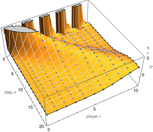
 precisely. Hence for a given player, the adjacent steps n = 2i – 2 and 2i – 1 are equally likely locations their game will be “discontinued”. This is surely the maximum assuming integer parameters, apart from the first player for whom step 0 is safe but step 1 is their most likely “resting place”. Hence the reader might prefer to translate our gaussian approximation by half a step or so; apparently there are various approximations to a binomial coefficient. The subsequent step n = 2i is a more likely endpoint than the earlier step 2i – 3.
![\[\sum_{n=1}^\infty n \cdot b_{i,n} = \binom{0}{i-1} \cdot {_2F_1}(1,-i,2-i;-1).\]](http://cmaclaurin.com/cosmos/wp-content/ql-cache/quicklatex.com-0f3dccf6f75fd13139f30b246197f5bb_l3.png "Rendered by QuickLaTeX.com")
![\[\sum_{i=1}^n b_{i,n} = \frac{1}{2}\]](http://cmaclaurin.com/cosmos/wp-content/ql-cache/quicklatex.com-96db9a287f5e5379a366181fa278d0e1_l3.png "Rendered by QuickLaTeX.com")
 is ½ times a binomial distribution in n. We previously found a gaussian curve for a given player i. Now. for a fixed step n, the de Moivre-Laplace approximation is a gaussian over the player number i:
![\[\frac{1}{\sqrt{2\pi(n-1)}}e^{-\frac{(i - n/2 - 1/2)^2}{(n - 1)/2}.\]](http://cmaclaurin.com/cosmos/wp-content/ql-cache/quicklatex.com-a116c9ac4435931ac0b441c0a434f974_l3.png "Rendered by QuickLaTeX.com")
 or equivalently P(i,n) for the probability the ith player is still alive on the nth step. We showed these probabilities satisfy the recurrence relation
  , along with initial conditions
  , and
, and  for all players after the first. Equivalently, we can start from
  , and
, and  for
for  . This is a bit like Pascal’s triangle. Rather than adding the previous two terms, we take their average — which of course is the sum divided by two. And rather than 1’s at the sides, we have 0’s and 1’s.
 . These values satisfy the same recurrence relation as before:
![\[\begin{aligned} b_{i,n} &=a_{i,n-1} - a_{i,n} \\ &= \frac{1}{2}(a_{i-1,n-2}+a_{i,n-2}-a_{i,n-1}-a_{i-1,n-1}) \\ &= \frac{b_{i,n-1}+b_{i-1,n-1}}{2}.\end{aligned}\]](http://cmaclaurin.com/cosmos/wp-content/ql-cache/quicklatex.com-da6343d9bf534f13b5dc03dfc1a22bc1_l3.png "Rendered by QuickLaTeX.com")
 , and
, and  for all players after the first. It is aesthetic to begin a step earlier:
  , except for
  . The Table below shows a few early entries.
 . For player i to die on step n, the previous i – 1 players must have died somewhere amongst the n – 1 prior steps. There are “n – 1 choose i – 1″ ways to arrange these mistaken steps, out of
  total combinations of equal probability. Given any such arrangement, the next player has a 50% chance their following leap is a misstep, hence:
![\[b_{i,n} := P(i\textrm{ dies on }n) = \binom{n-1}{i-1}2^{-n}.\]](http://cmaclaurin.com/cosmos/wp-content/ql-cache/quicklatex.com-aacd3fe49ce5a0492c0f36aef8ec97da_l3.png "Rendered by QuickLaTeX.com")
![\[P(i\textrm{ players died by }n) = \binom{n}{i}2^{-n}.\]](http://cmaclaurin.com/cosmos/wp-content/ql-cache/quicklatex.com-6d44375f1554e6a734df81effcf84eb8_l3.png "Rendered by QuickLaTeX.com")
 . Note if player i died on n′, the next player must make n – n′ correct guesses in a row, so that no-one else dies by the nth step.
 , which computer algebra simplifies to:
![\[P(i,n) = 1-\binom{n}{i}2^{-n}\cdot{_2F_1}(1,i-n,i+1;-1).\]](http://cmaclaurin.com/cosmos/wp-content/ql-cache/quicklatex.com-c2a20461aa048defc051d32943dbc8a9_l3.png "Rendered by QuickLaTeX.com")
 is called the “(ordinary) hypergeometric function”. I gave a limited table of these probability values in the previous blog. For fixed integer
  , the entire expression reduces to a polynomial in n of order i – 1 with rational coefficients, all times
 ![\[P(5,n) = 2^{-n}\frac{1}{24}\big( n^4-2n^3+11n^2+14n+24 \big).\]](http://cmaclaurin.com/cosmos/wp-content/ql-cache/quicklatex.com-65fec34ea05382f11c468a294e8a64cc_l3.png "Rendered by QuickLaTeX.com")
 , so players get some steps for free. The diagonal terms are
  . This makes sense because for player i to not be alive on the ith step, every leap by previous players must also have been a misstep. Some results like these may also be shown using induction and the recurrence relation. I give more special cases in the next blog post. Yet the general formula works even for non-integers, though this is not physical, as the Figure below shows. For negative parameters (not shown) it has a rich structure, with singularities, and some
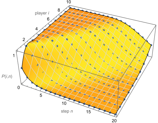
 , an exponential decrease. In the show (~30 minute mark), one player actually calculates this: 15 untested steps remain ahead of him, for a horrifyingly low 1/32768 chance of survival from that point. (Actually this is the third player, but more on that later.)
 .
. . Similar reasoning applies to any step up to n – 1. However if the first player is still alive on n – 1, their follower is guaranteed to reach step n successfully. (Any later performance of the first player is irrelevant to their successors at step n.) The overall probability is the sum over these possibilities, which for an arbitrary player is:
![\[a_{i,n} = a_{i-1,n-1} + \sum_{k=1}^{n-1} ( a_{i-1,k-1} - a_{i-1,k} ) / 2^{n-k}.\]](http://cmaclaurin.com/cosmos/wp-content/ql-cache/quicklatex.com-4d627692bbc0347df278931cf76ca111_l3.png "Rendered by QuickLaTeX.com")
 precisely.) Hence starting from the initial conditions given earlier, we may build up an array of values using a spreadsheet, computer program, or computer algebra system. The latter choice preserves exact fractions, which feels very satisfying. Also we define
  for convenience, where “step 0” may be interpreted as the ledge contestants safely start from. The Table below gives the first few values.
 , and the next player likely will:
  . In the show, 16 players compete in this challenge, so the last player has excellent odds, supposedly:
  . However our analysis does not account for human behaviour! In the show, time pressure, rivalries, and imperfect memory compete with logical decision making and the interests of the group as a whole. On the other hand, some players claim to distinguish the glass types by sight or sound, which would give an advantage. These make interesting plot elements, but would spoil the simplicity and purity of a mathematical analysis.
![\[a_{i,n} = \frac{a_{i,n-1} + a_{i-1,n-1}}{2}.\]](http://cmaclaurin.com/cosmos/wp-content/ql-cache/quicklatex.com-988bec155d8cf31b58464a852f4f5ebc_l3.png "Rendered by QuickLaTeX.com")
 to the previous step and previous player. [Update, 21st April: A simpler way is to consider step 1. If player 1 guesses breaks it, there are i – 1 remaining players for the next n – 1 steps. If player 1 instead guesses correctly, there are i players for the next n – 1 steps. This gives the recurrence relation.] Consider the three cases for player i – 1: they (A) died before step n – 1, (B) died on step n – 1, or (C) made it safely to step n – 1 or further. The total probability is the sum of these cases:
![\[P(i,n) = P(i,n|A)P(A) + P(i,n|B)P(B) + P(i,n|C)P(C).\]](http://cmaclaurin.com/cosmos/wp-content/ql-cache/quicklatex.com-79a6c7db91ab2e9fffdd1eb5ff39d90e_l3.png "Rendered by QuickLaTeX.com")
 . Hence the decomposition becomes:
![\[P(i,n) = \frac{1}{2}P(i,n-1|A)P(A) + \frac{1}{2}P(B) + P(C).\]](http://cmaclaurin.com/cosmos/wp-content/ql-cache/quicklatex.com-18ab8d3ca33850d7e04fd8ffd756f0d1_l3.png "Rendered by QuickLaTeX.com")
 apart from the C term, as seen from expanding out the conditional cases. Now
  . It follows
  as before. We did not need to evaluate P(A) or P(B), though this is straightforward.
 of surviving the bridge. This would seem to contradict the earlier calculation, which gave a lower chance by a factor of 21½, a surprising contrast! The black-masked “Front Man” said to the VIP observers, “I believe this next game will exceed your expectations” (~12:30 mark), but in this sense it did not 😆 . The distinction is the information learned. Conditional probability is a subtle and beautiful thing. If we know nothing about the previous attempts, nor the state of the bridge, the probabilities are our variables
  .
. , which might be interpreted physically as observers or a fluid. It may be useful to derive a time coordinate
  which both coincides with proper time for the observers, and synchronises them in the usual way. Here we consider only the geodesic and vorticity-free case. Define:
![\[dT := -\mathbf u^\flat.\]](http://cmaclaurin.com/cosmos/wp-content/ql-cache/quicklatex.com-1960cbec316fdccc06a33d0856d4b0cc_l3.png "Rendered by QuickLaTeX.com")
 . On the LHS,
  is the gradient of a scalar, which may be expressed using the familiar chain rule:
![\[dT = \frac{\partial T}{\partial x^0}dx^0 + \frac{\partial T}{\partial x^1}dx^1 + \cdots,\]](http://cmaclaurin.com/cosmos/wp-content/ql-cache/quicklatex.com-8e714fd4676c076ff9ae1e2f59d1ab91_l3.png "Rendered by QuickLaTeX.com")
 is a coordinate basis. Technically
  in the cobasis
  . Similarly
  , so we must match the components:
  . For our purposes we do not need to integrate explicitly, it is sufficient to know the original equation is well-defined. (No such time coordinate exists if there is acceleration or vorticity, which is a corollary of the Frobenius theorem, see Ellis+ 2012
 . One can show its change with proper time is
  . Further, the
  hypersurfaces are orthogonal to
  is parallel to
  -coordinate by
  . Similarly one new component is
  . Also
  , where
  . The
. The  are the same by symmetry, and the remaining components are unchanged. Hence the new components in terms of original components are:
![\[g'^{\mu\nu} = \begin{pmatrix} -1 & -u^1 & -u^2 & -u^3 \\ -u^1 & g^{11} & g^{12} & g^{13} \\ -u^2 & g^{21} & g^{22} & g^{23} \\ -u^3 & g^{31} & g^{32} & g^{33} \end{pmatrix}.\]](http://cmaclaurin.com/cosmos/wp-content/ql-cache/quicklatex.com-f2de30201432026fda1960ec99333f55_l3.png "Rendered by QuickLaTeX.com")
 . The 4-velocity components are:
  by the original equation. Also
  , and the
  are unchanged. Hence
  .
. , rearrange for
  , and substitute it into the original line element. This works but is clunky. My original inspiration was