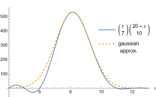
Gaussian approximation to a certain product of binomial coefficients

Difficulty: ★★★☆☆ undergraduate

Consider the following function, which is the product of a certain pair of binomial coefficients:

$f(x) := \binom{x}{a}\binom{X-x}{b}.$

We take a, b, X >> 1 to be constants, and x to have domain [a – 1, X – b + 1] which implies X > a + b – 2 at least. As usual $\binom{x}{a} := x!/a!(x-a)!$ , and this is extended beyond integer values by replacing each factorial with a Gamma function. Note the independent variable x appears in the upper entries of the binomial coefficients. Curiously, from inspection f is well-approximated by a gaussian curve. To gain some insight, for integer values of the parameters f is the polynomial:

$(a! b!)^{-1}x(x-1)\cdots(x-a+1)\cdot(X-b+1-x)\cdots(X-x).$

This has many zeroes, and sometimes oscillates wildly in between them, hence the domain of x specified earlier.

plot of function and a gaussian curve approximation — Figure: The function for a = 7, b = 10, and X = 20. It is shown beyond our stated domain, which is bounded by the roots at x = 6 and 11. The gaussian uses our estimated centre of x = 277/34 or approx. 8.147, whereas f‘s actual maximum occurs at around x = 8.139. The variance is from our approximate harmonic number formula, evaluated at the estimated centre point. Alternately, the “finite difference” derivatives give a poor estimate in this case. In general, the gaussian fit looks best for high parameter values with a near b, etc.

Now the usual approximations to a single binomial coefficient (actually, binomial distribution) are not helpful here. For example the de Moivre–Laplace approximation is a gaussian in terms of the lower entry in the binomial coefficient, whereas our x is in the upper entries. More promising is the approximation as a Poisson distribution, which leads to a polynomial which is itself gaussian-like, and motivated the previous post incidentally. However we proceed from first principles, by estimating the centre point and the second derivative there.

At the (central) maximum of f, the slope is zero. In general the derivative is $f'(x) = f(x)(H_x-H_{x-a}-H_{X-x}+H_{X-b-x})$ , where the H’s are called harmonic numbers. There may not exist any simple explicit expression for the turning points. Instead, the ratio of nearby points is comparatively simple:

$\frac{f(x-1/2)}{f(x+1/2)} = \frac{(x-a+1/2)(X+1/2-x)}{(x+1/2)(X-b+1/2-x)},$

using the properties of the binomial coefficient. The derivative is approximately zero where this ratio is unity, which occurs at:

$x_0 := \frac{2aX+a-b}{2(a+b)}.$

This should be a close estimate for the central turning point. [To do better, substitute specific numbers for the parameters, and solve numerically.] It is typically not an integer. Our sought-for gaussian has form $C\operatorname{exp}(-(x-x_0)^2/2\sigma^2)$ . We set the height $C := f(x_0)$ . Only the width remains to be determined. The gaussian’s second derivative evaluated at its centre point is $-C/\sigma^2$ . On the other hand:

$f''(x) = f'(x)^2/f(x) - (H_x^{(2)}-H_{x-a}^{(2)}+H_{X-x}^{(2)}-H_{X-b-x}^{(2)})f(x),$

which uses the so-called harmonic numbers of order 2, and I incorporate the function and its derivative (both given earlier) for brevity of the expression. Matching the results at $x_0$ yields the variance parameter $\sigma^2$ :

$\sigma^{-2} := H_{x_0}^{(2)}-H_{x_0-a}^{(2)}+H_{X-x_0}^{(2)}-H_{X-b-x_0}^{(2)},$

using $f'(x_0) \approx 0$ . (At large values the series $H_x^{(2)} \approx \pi^2/6 -1/x +1/2x^2\cdots$ may give insight into the above.) But alternatively, we can approximate the second derivative using elementary operations. By sampling the function at $x_0-1$ , $x_0$ , and $x_0+1$ say, a “finite differences” approach gives approximate derivatives. We can use the simple ratio formula obtained earlier to reduce the sampling to one or two points only, which might gain some insight along the way (though I currently wonder if this is a dead end…).

Now $f'(x_0-1/2) \approx f(x_0) - f(x_0-1)$ , which becomes:

$\frac{2C(a+b)^3}{(2aX+a-b)(2bX-2b^2-2ab+a+3b)},$

after using the ratio formula to obtain $f(x_0-1)$ in terms of C. Similarly it turns out $f'(x_0+1/2)$ is the negative of the above expression, but with a and b interchanged. Then a second derivative is: $f''(x_0) \approx f'(x_0+1/2)-f'(x_0-1/2)$ , but the combined expression does not simplify further so I won’t write it out. The last step is to set $\tilde\sigma^2 := -C/f''(x_0)$ , which is different to the earlier choice.

A slightly different approach uses $f'(x_0-1/2) \approx (f(x_0+1/2)-f(x_0-3/2))/2$ , which may be expressed in terms of another sampled point $E := f(x_0-1/2) = f(x_0+1/2)$ . Similarly $f'(x_0+1/2) \approx (f(x_0+3/2)-f(x_0-1/2))/2$ . The estimate for the second derivative follows, then later:

$\hat\sigma^2 := \frac{-2C(aX-b)(bX+a+2b)(bX-b^2-ab+a+2b)(aX-a^2-ab-b)}{E(a+b)^6}.$

The expression is a little simpler in this approach, but at the cost of a second sample point. The use of $f'(x_0-1) \approx f(x_0-1/2)-f(x_0-3/2)$ and $f'(x_0+1) \approx f(x_0+3/2)-f(x_0+1/2)$ instead leads to the same result.

Leave a Reply Cancel reply