Spatial gradient examples – CMacLaurin.com

Difficulty: ★★★☆☆ undergraduate

Last time we discussed the “spatial gradient” or “3-gradient”, and here we follow up with two examples. Recall from before that a scalar field $\Phi$ has gradient $d\Phi$ , and the part of this which is orthogonal to an observer 4-velocity $\mathbf u$ is, as a vector:

$^{(3)}(d\Phi)^\sharp := (d\Phi)^\sharp + \langle d\Phi,\mathbf u\rangle \mathbf u.$

This direction has the greatest increase of $\Phi$ , for any vector in $\mathbf u$ ’s 3-space (that is, orthogonal to $\mathbf u$ ), per length of the vector.

As an example, suppose the 4-gradient vector $(d\Phi)^\sharp$ is a null, future-pointing vector. It can be decomposed $E(\mathbf u+\boldsymbol\xi)$ , where $E := -\langle d\Phi,\mathbf u\rangle$ , and $\boldsymbol\xi$ is a unit spatial vector orthogonal to $\mathbf u$ . Physically, this gradient may be interpreted as a null wave or photon, which the observer determines to have energy (or related quantity, such as frequency) $E$ , and to move in the spatial direction $\boldsymbol\xi$ . The 3-gradient vector is $E\boldsymbol\xi$ , hence the direction of relative velocity also has the steepest increase of $\Phi$ , within the observer’s 3-space.

Suppose now $(d\Phi)^\sharp$ is a unit, timelike, future-pointing vector, so that we may interpret it as the 4-velocity $\mathbf v$ of a second observer. Then $^{(3)}(d\Phi)^\sharp = \mathbf v - \gamma\mathbf u$ , where $\gamma = - \langle\mathbf u,\mathbf v\rangle$ is the Lorentz factor between the pair. But we also have the “relative velocity” decomposition $\mathbf v = \gamma(\mathbf u + \mathbf V)$ , where $\mathbf V$ is the relative velocity of $\mathbf v$ as determined in $\mathbf u$ ’s frame, as I discussed previously. Combining these, $^{(3)}(d\Phi)^\sharp = \gamma\mathbf V$ . Hence within the observer’s 3-space, $\Phi$ again increases most sharply in the direction of the relative velocity.

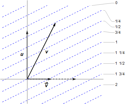Spacetime diagram, from the observer $\mathbf u$ ‘s perspective. The timelike 1-form $d\Phi \equiv \mathbf v^\flat$ is suggested by dotted blue lines, given at intervals of 1/4 for more resolution. These are orthogonal to the vector $\mathbf v$ , in the Lorentzian sense.

The figure shows the single tangent space — think of this as the linearisation of what is happening locally over the manifold itself. The hyperplanes are numbered by $\Phi$ , where only the differences between them are relevant, as an overall constant was not specified. Observe $\mathbf v$ crosses four of them, spanning an interval $\Delta\Phi = \langle d\Phi,\mathbf v\rangle = -1$ , so $\Phi$ is the negative of $\mathbf v$ ’s proper time; see a previous post for more background. In both our examples, the scalar decreases towards the future (or can vanish in the null case), even though the gradient vectors are future-pointing. That is, the gradient vectors actually point “down” the slope! This quirk is due to our −+++ metric signature, and would apply to spacelike gradients if +−−− were used instead. This really hurt my brain, until I drew the diagram. 🙁

To construct it, consider the action of $d\Phi$ on the axes. The horizontal axis is the relative velocity direction, with unit vector $\hat{\mathbf V} := \mathbf V/\beta$ . One can show $\langle d\Phi,\hat{\mathbf V}\rangle = \beta\gamma$ . Also $\langle d\Phi,\mathbf u\rangle = -\gamma$ , but I find it easier to think of: $\langle d\Phi,-\mathbf u\rangle = \gamma$ . These give the number of hyperplanes crossed by the unit axes vectors, then you can literally “connect the dots” since the 1-form is linear. In the figure $\beta = 1/2$ , so $\gamma \approx 1.15$ . (As for the 3-gradient, it vanishes in the $\mathbf u$ direction, hence $\mathbf u$ must cross no contours of $^{(3)}d\Phi$ . It would be drawn as vertical lines, with corresponding vector pointing to the right.)

Most of our discussion applies to arbitrary 1-forms, not just gradients which are termed exact 1-forms. I derived the work here independently, but the literature contains some similar material. It turns out Jantzen, Carini & Bini 1992 research paper (arXiv) §2 explicitly define the “spatial gradient”, as they most appropriately call it. A few textbooks discuss scalar waves, for which the 3-gradient vector is the wave 3-vector, which is orthogonal to the wavefronts within a given frame, as discussed shortly.

Leave a Reply Cancel reply