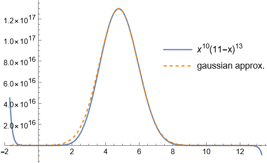
Gaussian approximation to a certain polynomial

Difficulty: ★★★☆☆ undergraduate

Consider the function:

$x^A(X-x)^B,$

where the independent variable x ranges between 0 and X, and the exponents are large: $A, B \gg 1$ . [We could call it a “polynomial”, though the exponents need not be integers. Specifically it is the product of “monomials” in x and X – x, so might possibly be called a “sparse” polynomial in this sense.] Surprisingly, it closely resembles a gaussian curve, over our specified domain $x \in [0,X]$ .

approximation to a certain polynomial using a gaussian curve — Figure: The polynomial with parameters A = 10, B = 13, and X = 11. Our gaussian approximation is visually indistinguishable near the centre. Outside our specified domain the polynomial tends to $\pm\infty$ , and for each non-integer exponent the tail on one side becomes imaginary.

The turning point is where the derivative equals zero. This occurs when x is the surprisingly simple expression:

$\tilde x := \frac{X}{1+B/A},$

at which the function has value:

$A^A B^B \Big(\frac{X}{A+B}\Big)^{A+B} \equiv (B/A)^B \tilde x^{A+B}.$

An arbitrary gaussian, not necessarily normalised, has form: $Ce^{-(x-D)^2/2\sigma^2}$ . This has centre D which we equate with $\tilde x$ , and maximum height C which we set to the above expression. We can fix the final parameter, the standard deviation, by matching the second derivatives at the turning point. Hence the variance is:

$\sigma^2 = \frac{AB}{(A+B)^3}X^2 \equiv \frac{B}{A^2X}\tilde x^3.$

Hence our gaussian approximation may be expressed:

$\boxed{(B/A)^B \tilde x^{A+B} \operatorname{exp}\Big( -\frac{(x-\tilde x)^2}{2B\tilde x^3/A^2X} \Big).}$

The integral of the original curve turns out to be:

$\int_0^X x^A(X-x)^Bdx = \frac{X^{A+B+1}}{(A+B+1)\binom{A+B}{A}}.$

This uses the binomial coefficient $\binom{A+B}{A} := (A+B)!/A!B!$ , which is extended to non-integer values by replacing the factorials with Gamma functions. We could then apply Stirling’s approximation $A! \approx \sqrt{2\pi A}(A/e)^A$ to each factorial, to obtain:

$\int\cdots \approx \frac{\sqrt{2\pi(A+B)}}{A+B+1}(B/A)^{B+1/2}\tilde x^{A+B+1},$

though this is more messy to write out. On the other hand, the integral of the gaussian approximation is:

$\int_{-\infty}^\infty \operatorname{exp}\cdots = \sqrt\frac{2\pi}{A+B}(B/A)^{B+1/2}\tilde x^{A+B+1}.$

We evaluated this integral over all real numbers, because the expression is simpler and still approximately the same. The ratio of the above two expressions is $(A+B)/(A+B+1) \approx 1$ .

Leave a Reply Cancel reply