Gradient of a scalar

Difficulty: ★★★☆☆ undergraduate

Suppose a scalar field $\Phi$ is defined on some region of spacetime. Its gradient $d\Phi\equiv \nabla\Phi$ expresses the change in $\Phi$ (that is, its derivative) in each direction. In a coordinate system, it has components:

$\nabla_\mu\Phi = (d\Phi)_\mu = \Phi_{,\mu} := \frac{\partial\Phi}{\partial x^\mu}.$

$d\Phi$ is a 1-form or covector. [Recall a 1-form is just a (0,1)-tensor. Schutz 2009 book also uses the term dual vector, though I find this can lead to clumsy wording, such as the hypothetical phrase: “the vector [which is] dual to a dual vector”. Traditionally the term covariant vector has been used, meaning its components transform “covariantly” with a change of basis. 1-forms are a rigorous version of differentials, superceding the older idea of infinitesimals but using similar notation (Schutz 1980 book §2.19; Spivak vol. 1 book §4).] Above, “ $d$ ” is called the exterior derivative, and $\nabla$ is the covariant derivative, but when acting on a scalar these coincide. Recall a 1-form accepts a vector and returns a number. In this case, the vector is the direction of differentiation, and the output is the derivative of $\Phi$ in that direction (where the vector’s magnitude matters also).

The 1-form $d\Phi$ may be visualised as a set of hypersurfaces or level sets $\Phi = \textrm{const}$ , on the manifold (MTW book §2.5–2.7, Box 4.4; Schutz 2009 §3.3). Ideally these could be spaced at intervals $\Delta\Phi = 1$ . Given some vector $\mathbf Y$ , the contraction:

$d\Phi(\mathbf Y) \equiv \langle d\Phi,\mathbf Y\rangle = Y^\mu\frac{\partial\Phi}{\partial x^\mu}$

is visualised as the number of hypersurfaces the vector pierces, or “bongs of [a] bell” in MTW’s colourful terminology. Technically however, vectors and 1-forms exist in the (co-)tangent spaces, not extended along the manifold. At any given point, $d\Phi$ is the linear approximation to $\Phi$ , ignoring the constant term (MTW §2.6). Hence $d\Phi$ is more accurately visualised as hyperplanes within the tangent space there. The diagram below shows both artistic choices. Note in two dimensions, hypersurfaces and hyperplanes are just curves and straight lines, respectively.

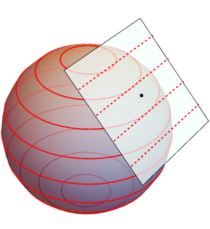
sphere with dtheta field — A 2-sphere with visualisations of the 1-form field $d\theta$ , both over the entire manifold and within a single tangent space. The spacing is $\Delta\theta = \pi/10$ .

The gradient vector is the dual to $d\Phi$ , with components obtained by raising the index in the usual way: $g^{\mu\nu}(d\Phi)_\nu$ . This may be elegantly written $(d\Phi)^\sharp$ , where the “sharp” symbol is part of the “musical isomorphism” notation. While the gradient is usually first encountered as a vector, it is most naturally a 1-form, as this does not require a metric (MTW §9.4). As Schutz 2009 §3.3 explains:

…we in general cannot call a gradient a vector. We would like to identify the vector gradient as that vector pointing ‘up’ the slope, i.e. in such a way that it crosses the greatest number of contours per unit length. The key phrase is ‘per unit length’. If there is a metric, a measure of distance in the space, then a vector can be associated with a gradient. But the metric must intervene here in order to produce a vector. Geometrically, on its own, the gradient is a one-form.

But if one does not know how to compare the lengths of vectors that point in different directions, one cannot define a direction of steepest ascent…

The last line is from Schutz 1980 §2.19, where the discussion is similar. These textbooks give a superb introductory account of 1-forms, however the steepness comments are only valid for a Riemannian metric, with positive-definite signature. Consider Minkowski spacetime with coordinates $(t,x,y,z)$ . By linearity, we need only consider unit vectors. The 1-form $dx$ has components $(0,1,0,0)$ , with $(dx)^\sharp$ just $\partial_x$ . These contract to give unity. If we restrict to vectors spanned by $\partial_x$ , $\partial_y$ and $\partial_z$ , Schutz’ steepness comments apply. However $\pm(\beta\gamma,\gamma,0,0)$ is also a unit spacelike vector, where $\gamma = (1-\beta^2)^{-1/2}$ , but combines with $dx$ to give $\pm\gamma$ , hence crosses more intervals $x = \textrm{const}$ than the gradient vector does. Similarly for $dt$ , the contraction with $(dt)^\sharp = -\partial_t$ returns $-1$ , but with the unit timelike vector $\pm(\gamma,\beta\gamma,0,0)$ yields $\pm\gamma$ . Hence for a timelike 1-form, its gradient vector crosses the least contours (taking the absolute value) per unit length, compared to other timelike vectors only. For a null 1-form, its gradient vector lies along the hyperplanes, so crosses zero of them (MTW Figure 2.7)!

Instead, we are left with saying the gradient vector is orthogonal to all vectors $\mathbf Y$ on which the 1-form vanishes: $\langle (d\Phi)^\sharp,\mathbf Y\rangle = 0$ whenever $\langle d\Phi,\mathbf Y\rangle = 0$ . The angle brackets mean contraction using the metric, with indices appropriately raised or lowered. Another property is the gradient vector’s squared-norm equals the 1-form’s squared-norm, which also matches the number of contours crossed:

$\langle (d\Phi)^\sharp,(d\Phi)^\sharp\rangle = \langle d\Phi,d\Phi\rangle = \langle d\Phi,(d\Phi)^\sharp\rangle.$

The above statements are basically tautologies, but they help clarify what metric duality means. Incidentally, not all 1-forms arise as the “ $d$ ” of a scalar, but only those termed exact (Wald book §B1). Most of this post applies also to arbitrary 1-forms $\boldsymbol\alpha$ , for which the hyperplanes are spanned by vectors satisfying $\langle\boldsymbol\alpha,\mathbf Y\rangle = 0$ . For many creative illustrations see MTW, including their “honeycomb” and “egg crate” analogies for 2-forms and 3-forms, and their Figure 4.5 for the 2-form $d\theta\wedge d\phi$ . Finally, I previously reviewed contractions like $d\Phi(\mathbf u) = d\Phi/d\tau$ , which give the rate of change of the scalar by proper time along a worldline.

One thought on “Gradient of a scalar”

Leave a Reply Cancel reply