In relativity, distances and times are relative to an observer’s velocity. Hence one should be careful when defining an angular momentum. Speaking generally, a natural parametrisation of 4-velocities uses Killing vector fields, if the spacetime has any. In Schwarzschild spacetime, Hartle (2003 §9.3) defines the Killing energy per mass and Killing angular momentum per mass as:
The angle brackets are the metric scalar product, has range , and we will take to be a 4-velocity. I have relabeled Hartle’s as . While and are just coordinate basis vectors for Schwarzschild coordinates, as Killing vector fields (KVFs) they have geometric significance beyond this convenient description. [ is the unique KVF which as in “our universe” (region I), is future-pointing with squared-norm . On the other hand has squared-norm , so is partly determined by having maximum squared-norm amongst points at any given , which implies it is orthogonal to , although the specific orientation is not otherwise determined geometrically.]
In fact is the portion of angular momentum (per mass) about the -axis. In Cartesian coordinates , the KVF has components . Similarly, we can define angular momentum about the -axis using the KVF , which in spherical coordinates is . For the -axis we use , which is in the original coordinates. Then:
Hence we can define the total angular momentum as the Pythagorean relation , that is:
This is a natural quantity determined from the geometry alone, unlike the individual etc. which rely on an arbitrary choice of axes. It is non-negative. I came up with this independently, but do not claim originality, and the general idea could be centuries old. Similarly quantum mechanics uses and , which I first encountered in a 3rd year course, although these are operators on flat space.
One 4-velocity field which conveniently implements the total angular momentum is:
In this case the axial momenta are , , and , for a total Killing angular momentum as claimed. There are restrictions on the parameters, in particular the “” must be a minus in the black hole interior. Incidentally this field is geodesic since . It also has zero vorticity (I wrote a technical post on the kinematic decomposition previously), so we might say it has macroscopic rotation but no microscopic rotation. Another possibility is in terms of and :
where the first two components are the same as the previous vector. The expressions are simpler with a lowered index .
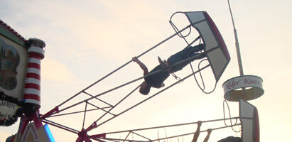
Possibly my favourite amusement park ride I have ever tried was called a Schiffschaukel, which is German for “ship swing”. It was powered only by the rider, with no motor of any kind. With enough skill, you could make a complete 360° vertical loop! In place of the rope or chain links in an ordinary swing, it was supported by rigid struts, which helped achieve a complete rotation. I loved the physical challenge of it. It was easy to start it rocking. I also managed to get my body above the horizontal, but not to make a complete loop. However one man I watched could not only achieve a loop, but gauged his speed so as to hang upside down for a few seconds, neck craned forward to watch the ground, before he gradually tipped over.
Schiffschaukel or ship swing, from Oktoberfest.net. The one I rode was in a local Volksfest (“people’s festival”) in a town outside of Munich, in 2007. It looked a lot like the one in this photo, with a few cosmetic differences: as I recall I had no waist harness but just one foot strapped in, there were two supporting struts rather than four, no “boat” decoration, and the swing was shorter.
In my experience most people, including Germans, have never heard of it. Wikipedia calls it a “ship swing”, in contrast to a “pirate ship” ride which is motorised. I have been on a couple of the latter rides in Australia: huge structures which seat dozens of people, and are quite different to the self-propelled swing. The unpowered type date from the 1800s apparently; many held two people, and had ropes to pull on. The German language Wikipedia has more information: here is an automatic translation. Also it turns out there is a modern Estonian sport kiiking (meaning “swinging”) which is the same concept. The current world record for a revolution is a swing with radius just over 7 metres, achieved by an Olympic medal-winning rower.
But how is it even possible to make a loop? I found it counter-intuitive, like pulling yourself up by the bootstraps, as the proverbial saying goes. Similarly, I recently learned of “pump tracks” for bicycles, from my brother. It is possible to propel yourself around such a course, which consists of mounds and banked corners, without pedalling! The energy comes from raising or lowering your body with the correct timing. In fact you can even propel yourself on flat ground this way, by making appropriate turns and body maneuvers.
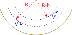
Conservation of angular momentum along a circular arc. The rider travels from left to right, with their centre of mass initially following the middle arc. After standing up, their centre of mass follows the inner arc, and their velocity is increased. (The solid arc is the ground or base of the ship, say.)
Conservation of angular momentum explains both scenarios. Consider a circular, concave segment of track, as with the ship swing. Approximate the person, plus bike or “ship”, as a point object with mass . Suppose this point, their centre-of-mass, moves on a circle with radius (note this is less than the radius of the track arc). The angular momentum, as determined from the centre of curvature, is , where is the speed. (Technically this is a vector cross-product, but in this simple example where the vectors are at 90°, we can more or less treat it as an ordinary multiplication of numbers.) Now suppose the rider stands up straighter, so their centre of mass moves a “height” towards the centre of curvature. The angular momentum is , where is the new speed. But since angular momentum is conserved, this must match the previous expression, hence:
The speed has increased! Note the rider put work in, by not only resisting the centrifugal acceleration , but moving against it, in the opposite direction. The forces can be severe. For a swing to barely reach the top, it must have a speed at the bottom of the arc, by conservation of kinetic and gravitational potential energy. Here is the “acceleration” due to gravity. The centripetal acceleration at the lowest part is , which is independent of the radius. Including the weight due to gravity gives a total of — that is, a g-force of 5!
The swing rider should probably bend their knees when reaching the maximum height of their arc, to reverse the process and complete the cycle. If their speed is zero at this point (so a full revolution is not achieved), crouching has no effect on the speed, which is zero after all. In this case the maximum speed — measured when at the lowest part of the circle — grows by the fixed proportion with each swing. This is exponential growth! Once revolution is achieved, the rider can gain further speed by crouching at the top of the circle. While this reduces their speed by the same proportion , over one revolution there is a net gain, since the speed at the bottom is greater due to gravitational fall.
1/2 m Vlow^2 = mg2R + 1/2 m Vtop^2
Vlow^2 = 4gR + Vtop^2
If Vtop is speed before crouch, then should really use Vtop/ratio. So:
Vlow^2*ratio^2 = 4gR + Vtop^2/ratio^2
Suppose speed V just before bottom. Then V*ratio after standing. At top, before crouch, Vtop^2 = V^2*ratio^2 – 4gR. After crouch, new speed^2 is: Vtop^2/ratio^2 = V^2 – 4gR/ratio^2. At bottom, before standing, Vlow^2 = V^2 + 4gR(1-1/ratio^2).
So with each revolution, the kinetic energy increases by a fixed amount (not fixed proportion). This is linear growth. Hence the speed increases indefinitely, but slowing rate. Of course this ignores friction, the rider’s strength, etc., assumes instantaneous repositioning
On a pump track the strategy is analogous: in a valley you should stand up, and over a bump you should crouch down, as one webpage explains. In both cases you move closer to the centre of curvature. In internet forums, people say similar motions arise naturally in skateboarding, surfing, snowboarding, and other sports. Returning to the ship swing, I was not told any strategy at the time. On certain swings I sensed my speed diminish, so knew I had made a mistake. At the bottom of the swing, when the sum of centrifugal force and gravity is maximum, it felt safer to “go with the flow”, and unnatural to resist. But resist is exactly what I should have done.
Suppose you have an axially symmetric vector field. Can we define an affine connection which keeps the vectors “parallel”, under rotation about the axis? For example, we wish the vectors illustrated below to get parallel-transported around the circle:
We seek an affine connection which declares vectors at a given radius “parallel”, for any vector field with circular symmetry / cylindrical symmetry / rotational symmetry.
Take Minkowski spacetime in cylindrical coordinates , with metric , and consider a vector field whose components are independent of :
The covariant derivative in the tangential direction has components:
We want this to vanish, but first a quick recap (Lee §4, 5). Recall a connection is defined by , in terms of our coordinate vector frame . This extends to a covariant derivative of arbitrary vectors and tensors, also denoted “”. The derivative of above assumed the Levi–Civita connection, which is inherited from the metric: it is the unique symmetric, metric-compatible connection. In that case the set of are called Christoffel symbols, but in general they are called connection coefficients.
The offending Christoffel symbols which prevent our vector field from being parallel-transported are: and . But we are free to simply define a new connection for which these vanish: ! Given a frame, any set of smooth functions yields a valid connection (Lee, Lemma 4.10). It is natural to hold on to the other Christoffel symbols, to accord whatever respect remains for the metric. In fact only one is nonzero, . To set this to zero would essentially deny the increase in circumference with the radius. Incidentally, even with keeping , the new connection is flat, meaning its associated Riemann curvature tensor vanishes.
The new connection may be expressed as the Levi–Civita one with a bilinear correction:
where and are arbitrary vectors, to be substituted into the 2nd and 3rd slots respectively of the (1,2)-tensor in parentheses. This is much simpler than it looks, as the terms just pick out and -components, and return basis vectors. Equivalently, the correction may be written , where the angle brackets mean contraction of a 1-form and vector. Notice from here and the two “offending” Christoffel symbols mentioned earlier, that only (the component of) the derivative in the –direction is affected.
These expressions obscure some beautiful symmetry. Let’s raise one index and lower another, in the correction term:
Here is a wedge product, is just the 1-form with components , and “” is a contraction. The correction’s components are simply . This is a vector, even though some lowered indices appear in the expression. The correction is just a rotation in the –plane! From inspection of the diagram, this is unsurprising.
This is analogous to Fermi–Walker transport. Given a worldline, this corrects the (Levi–Civita connection) time-derivative by a rotation in the plane spanned by and the 4-acceleration vector . Under Fermi–Walker transport, orthonormal frames stay orthonormal over time, and their orientation agrees with gyroscopes. For both our connection and the Fermi-Walker derivative, there is a preferred differentiation direction, along which a rotation is added to the Levi-Civita derivative.
I previously wrote about a connection for a spherically symmetric vector field. This has been a good learning experience about connections other than Levi-Civita. Many of us completed general relativity courses in which the curvature quantities were merely formulae with no intuitive understanding. However questions from mathematicians like: “Which connection are you using?” prompted me to learn more. (At least I have never been asked which differential structure I am using, nor which point-set topology, which is fortunate for all involved. 🙂 ) There are various physically-motivated connections defined in research paper §2. I intend to apply this to the rotating disc, and to an observer field in Schwarzschild spacetime. Also, I accidentally came across Rothman+ 2001 about parallel transport in Schwarzschild spacetime, with numerous followup papers by various authors. All of this struck me again with a sense of fascination about curvature: how rich and deep it is.
The Lorentz boost between two reference frames can be expressed as a (1,1)-tensor , interpreted as an operator on vectors. Here we re-express this well known fact using a general, index-free, coordinate-independent, 4-vector notation, which is valid locally in curved spacetime.
Recall the prototypical Lorentz boost on Minkowski spacetime:
This is a boost in the -direction by speed or Lorentz factor. It maps an arbitrary vector to . Numerous authors generalise to arbitrary boost directions, such as Møller §18; MTW §2.9; or Tsamparlis §1.7. This typically involves separate transformations of time and 3-dimensional space: and . The arrows signify 3-dimensional vectors, is the position in 3-space, and is the relative 3-velocity. The space part uses beautiful, coordinate-independent vector language. However the time part requires privileged coordinates adapted to the observers. We will derive a 4-vector analogue.
Consider two 4-velocity vectors and (located at the same point, if in curved spacetime). They are related by the Lorentz boost:
where , the unit vector points in the boost direction, and is the relative velocity. This is the 4-vector analogue of the familiar coordinate boost . Combined with the space boost given shortly, this forms a local Lorentz transformation. While the plus sign makes the above appear an inverse boost, this is only because vectors (as whole entities) transform inversely to coordinates. Rearranging:
This is the relative velocity of the observer as determined in ’s frame, as explained previously. It is equivalent to the introduced in the 3-dimensional spatial transformation, except now treated as a 4-vector. It is orthogonal to , with length . Conversely, the relative velocity of as determined in ’s frame is . Now, the vector analogue of the usual boosted spatial coordinate is . After multiplying by :
Hence the relative velocity vectors are boosted into one-another, aside from a minus sign (Jantzen+ 1992 §4). This generalises the Newtonian result . So we have the boost’s action on the orthogonal vectors and , plus it is the identity on the 2-dimensional spatial plane orthogonal to both, hence:
using and . It is a good exercise to check the contractions with , , or any orthogonal to both. In index-free notation,
The “flat” symbol just means: lower an index. Equivalently, in terms of the initial observer and boost velocity alone:
in which case the relative speed may be obtained from . This is equivalent to MTW’s Exercise 2.7 which uses Cartesian coordinates, after adjusting various minus signs because I use vectors not vector components. In terms of the 4-velocities alone, we have the curiously symmetric expression:
Formulae are useful machines, allowing you to blithely turn the handle to crank out a result. This contrasts with my usual emphasis on conceptual understanding, and drawing a picture (at least mentally). However Lorentz boosts have many counter-intuitive or seemingly paradoxical effects. It is easier to make a mistake if you reason from first-principles alone. Of course the algebra does originate from careful thinking about foundations, and having multiple approaches is a check of consistency.
Boosts are paramount for comparing physical quantities between frames. Some textbooks present the general Lorentz boost in Minkowski spacetime with Cartesian coordinates. Our abstract vector formulation allows direct application to local boosts in arbitrary spacetime, such as Kerr or FLRW, in any coordinate system. I don’t remember seeing the formulae here in the literature, but someone should have done it somewhere. The Jantzen+ paper was an inspiration, and the same authors define various further quantities (projections, in fact) in Bini+ 1995.
Last time we discussed the “spatial gradient” or “3-gradient”, and here we follow up with two examples. Recall from before that a scalar field has gradient , and the part of this which is orthogonal to an observer 4-velocity is, as a vector:
This direction has the greatest increase of , for any vector in ’s 3-space (that is, orthogonal to ), per length of the vector.
As an example, suppose the 4-gradient vector is a null, future-pointing vector. It can be decomposed , where , and is a unit spatial vector orthogonal to . Physically, this gradient may be interpreted as a null wave or photon, which the observer determines to have energy (or related quantity, such as frequency) , and to move in the spatial direction . The 3-gradient vector is , hence the direction of relative velocity also has the steepest increase of , within the observer’s 3-space.
Suppose now is a unit, timelike, future-pointing vector, so that we may interpret it as the 4-velocity of a second observer. Then , where is the Lorentz factor between the pair. But we also have the “relative velocity” decomposition , where is the relative velocity of as determined in ’s frame, as I discussed previously. Combining these, . Hence within the observer’s 3-space, again increases most sharply in the direction of the relative velocity.
Spacetime diagram, from the observer ‘s perspective. The timelike 1-form is suggested by dotted blue lines, given at intervals of 1/4 for more resolution. These are orthogonal to the vector , in the Lorentzian sense.
The figure shows the single tangent space — think of this as the linearisation of what is happening locally over the manifold itself. The hyperplanes are numbered by , where only the differences between them are relevant, as an overall constant was not specified. Observe crosses four of them, spanning an interval , so is the negative of ’s proper time; see a previous post for more background. In both our examples, the scalar decreases towards the future (or can vanish in the null case), even though the gradient vectors are future-pointing. That is, the gradient vectors actually point “down” the slope! This quirk is due to our −+++ metric signature, and would apply to spacelike gradients if +−−− were used instead. This really hurt my brain, until I drew the diagram. 🙁
To construct it, consider the action of on the axes. The horizontal axis is the relative velocity direction, with unit vector . One can show . Also , but I find it easier to think of: . These give the number of hyperplanes crossed by the unit axes vectors, then you can literally “connect the dots” since the 1-form is linear. In the figure , so . (As for the 3-gradient, it vanishes in the direction, hence must cross no contours of . It would be drawn as vertical lines, with corresponding vector pointing to the right.)
Most of our discussion applies to arbitrary 1-forms, not just gradients which are termed exact 1-forms. I derived the work here independently, but the literature contains some similar material. It turns out Jantzen, Carini & Bini 1992 §2 explicitly define the “spatial gradient”, as they most appropriately call it. A few textbooks discuss scalar waves, for which the 3-gradient vector is the wave 3-vector, which is orthogonal to the wavefronts within a given frame, as discussed shortly.
Suppose you have a scalar field , and at a given point in spacetime: a 4-velocity vector interpreted as an “observer”. In which direction does increase most steeply, when restricted to the observer’s local 3-dimensional space?
Last time I reviewed the gradient 1-form or covector , and its associated gradient vector obtained by raising the index as usual. The gradient vector has been described as the direction of greatest increase in per unit length (Schutz 2009 §3.3). However this is only guaranteed when the metric is positive definite, meaning a Riemannian manifold, rather than a Lorentzian manifold as used to model spacetime.
The observer’s 4-velocity splits vectors and 1-forms into purely “time” parts parallel to , and purely “space” parts orthogonal to it. (Intuitively, it may help to think of a basis adapted to the observer, meaning , and the vectors are orthogonal to , where . Then a purely spatial vector is spanned by the . Since vectors and covectors are linear, we need only specify their values on a basis set.)
Consider the tangent space at the specified point. Imagine working within the observer’s local 3-space, by which I mean the 3-dimensional subspace consisting of vectors orthogonal to . Label the gradient as restricted to this subspace by . On the subspace the metric has Riemannian signature, hence the corresponding vector is the direction of steepest increase. We can mimic this mathematically by staying in 4 dimensions, but setting the “time” part to zero:
This is a 4-dimensional object, but I reuse the notation “” to imply it vanishes in the observer’s time direction. This “3-gradient” is the projection of orthogonal to . The angle brackets signify contraction of the 1-form and vector, and the “flat” symbol denotes the 1-form obtained from by “lowering the index” using the metric. The vector 3-gradient is:
This follows from “raising the index” using the inverse metric as usual. Note that on the subspace, the inverse metric coincides with the inverse 3-metric which has components , for . Equivalently, one can apply the spatial projector to either or , with the same result. This projector agrees with the inverse metric on the 3-space, and is zero on purely timelike covectors. Either way, the essential part of the process is to remove the “time” component of the gradient. I will give examples in the following post.
Suppose a scalar field is defined on some region of spacetime. Its gradient expresses the change in (that is, its derivative) in each direction. In a coordinate system, it has components:
is a 1-form or covector. [Recall a 1-form is just a (0,1)-tensor. Schutz 2009 also uses the term dual vector, though I find this can lead to clumsy wording, such as the hypothetical phrase: “the vector [which is] dual to a dual vector”. Traditionally the term covariant vector has been used, meaning its components transform “covariantly” with a change of basis. 1-forms are a rigorous version of differentials, superceding the older idea of infinitesimals but using similar notation (Schutz 1980 §2.19; Spivak vol. 1 §4).] Above, “” is called the exterior derivative, and is the covariant derivative, but when acting on a scalar these coincide. Recall a 1-form accepts a vector and returns a number. In this case, the vector is the direction of differentiation, and the output is the derivative of in that direction (where the vector’s magnitude matters also).
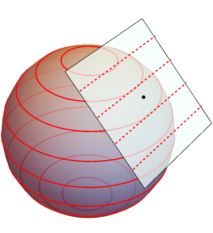
The 1-form may be visualised as a set of hypersurfaces or level sets , on the manifold (MTW §2.5–2.7, Box 4.4; Schutz 2009 §3.3). Ideally these could be spaced at intervals . Given some vector , the contraction:
is visualised as the number of hypersurfaces the vector pierces, or “bongs of [a] bell” in MTW’s colourful terminology. Technically however, vectors and 1-forms exist in the (co-)tangent spaces, not extended along the manifold. At any given point, is the linear approximation to , ignoring the constant term (MTW §2.6). Hence is more accurately visualised as hyperplanes within the tangent space there. The diagram below shows both artistic choices. Note in two dimensions, hypersurfaces and hyperplanes are just curves and straight lines, respectively.
A 2-sphere with visualisations of the 1-form field , both over the entire manifold and within a single tangent space. The spacing is .
The gradient vectoris the dual to , with components obtained by raising the index in the usual way: . This may be elegantly written , where the “sharp” symbol is part of the “musical isomorphism” notation. While the gradient is usually first encountered as a vector, it is most naturally a 1-form, as this does not require a metric (MTW §9.4). As Schutz 2009 §3.3 explains:
…we in general cannot call a gradient a vector. We would like to identify the vector gradient as that vector pointing ‘up’ the slope, i.e. in such a way that it crosses the greatest number of contours per unit length. The key phrase is ‘per unit length’. If there is a metric, a measure of distance in the space, then a vector can be associated with a gradient. But the metric must intervene here in order to produce a vector. Geometrically, on its own, the gradient is a one-form.
But if one does not know how to compare the lengths of vectors that point in different directions, one cannot define a direction of steepest ascent…
The last line is from Schutz 1980 §2.19, where the discussion is similar. These textbooks give a superb introductory account of 1-forms, however the steepness comments are only valid for a Riemannian metric, with positive-definite signature. Consider Minkowski spacetime with coordinates . By linearity, we need only consider unit vectors. The 1-form has components , with just . These contract to give unity. If we restrict to vectors spanned by , and , Schutz’ steepness comments apply. However is also a unit spacelike vector, where , but combines with to give , hence crosses more intervals than the gradient vector does. Similarly for , the contraction with returns , but with the unit timelike vector yields . Hence for a timelike 1-form, its gradient vector crosses the least contours (taking the absolute value) per unit length, compared to other timelike vectors only. For a null 1-form, its gradient vector lies along the hyperplanes, so crosses zero of them (MTW Figure 2.7)!
Instead, we are left with saying the gradient vector is orthogonal to all vectors on which the 1-form vanishes: whenever . The angle brackets mean contraction using the metric, with indices appropriately raised or lowered. Another property is the gradient vector’s squared-norm equals the 1-form’s squared-norm, which also matches the number of contours crossed:
The above statements are basically tautologies, but they help clarify what metric duality means. Incidentally, not all 1-forms arise as the “” of a scalar, but only those termed exact (Wald §B1). Most of this post applies also to arbitrary 1-forms , for which the hyperplanes are spanned by vectors satisfying . For many creative illustrations see MTW, including their “honeycomb” and “egg crate” analogies for 2-forms and 3-forms, and their Figure 4.5 for the 2-form . Finally, I previously reviewed contractions like , which give the rate of change of the scalar by proper time along a worldline.
Suppose you have a spherically symmetric vector field, as in the diagram. Can we find an affine connection which transports the vectors into one-another? That is, a geometry in which they are all “parallel”?
The vectors (red arrows) are clearly not parallel in the usual sense. But can we define a new connection in which they are transported into one-another?
Take Schwarzschild spacetime, in the usual coordinates . The coordinate basis vectors are , , , and . I will write these as , so for for example, this is the vector with components . Recall a connection is defined by:
where the are the connection coefficients, also called Christoffel symbols in the specific case of the Levi-Civita connection. (Recall the Levi-Civita connection is the one inherited from the metric: it is the unique symmetric and metric-compatible connection.) For each pair , this definition is interpreted as the derivative of the field, in the direction .
Now consider an arbitrary vector field of the form:
We would not expect the sought-for parallel transport to work for vectors with components in the or -directions — at least, not without imposing extra choices. In particular, the “hairy ball theorem” states no smooth, non-vanishing vector field along the 2-sphere exists: that is, within its 2-dimensional tangent bundle. For Schwarzschild spacetime, we move around a 2-sphere of constant and , by taking “directional derivatives” along the -plane. As expected, does not vanish, even in these directions:
The offending Christoffel symbols turn out to be and . These arise from and . These quantify how the radial coordinate vector changes as you move around on a sphere.
One option is to simply define new connection coefficients for which these vanish: and , and keep the remaining Christoffel symbols, in order to remain as close as possible to the metric connection. This procedure is justified, because given a frame field, any choice of smooth functions yields a valid connection (Lee 2018 , Introduction to Riemannian manifolds, Lemma 4.10). We can also write this new connection as the usual (Levi-Civita) covariant derivative plus a bilinear correction:
The parenthetical term is a (1,2)-tensor we interpret as accepting the vectors in the last two slots ( in the second slot, and into the last), returning another vector. The correction term may also be written , where the angle brackets mean contraction of a 1-form and vector in this case. Intuitively, the parenthetical term just above is also a projection, returning only the angular part of the differentiation direction . This is the blue arrow in the original diagram. For large , the basis vectors and grow very large, but the red vectors must adjust only by the angle rotated through, hence the multiplier. returns the radial component .
As a check, as required. The new connection is not symmetric, because and remain non-vanishing. Hence the connection has “torsion”. I won’t write out its Riemann and Ricci tensors, but the scalar curvature is ! At face value this violates the Einstein field equations, for which the Ricci tensor (and hence the scalar curvature) always vanish in a vacuum, however Einstein’s equations use the Levi-Civita connection. Curiously, the value is precisely the scalar curvature for a 2-sphere.
We can also construct a symmetric connection for which additionally . In the (somewhat) index-free expression:
where is the symmetric product, and analogously for . This connection has Ricci tensor equal to the metric in the and components, apart from a scalar factor , and vanishing elsewhere. Its scalar curvature is .
Hence we have constructed connections which parallel transport our spherically symmetric vector field around a sphere, and deviate as little as possible from the Levi-Civita connection. Neither of the new connections are “metric-compatible”, for instance . Hence . The same holds for .
If you find some formulae here do not work for you, compare your convention for the connection coefficient index order, or try swapping and in the correction terms. I had problems myself, so undertook a painstaking review of my own conventions, and wrote a new page describing them. Finally, beware of coordinate basis vectors! The “vectors” and actually depend on all four coordinates, which is related to the so-called “second fundamental confusion of calculus”! In case of ambiguity, perhaps some should be replaced with and , or scalar multiples thereof. I avoided this technicality in the interests of readability. This concern only applies to coordinate systems in which the metric is non-diagonal.
Difficulty: ★☆☆☆☆ no science: just travel, diary or musings
One of my favourite astrophysical phenomena was the appearance of the same supernova at various different times and places in the sky. The light from “Supernova Refsdal” was bent by a cluster of galaxies, whose gravity acted like a magnifying glass. This “gravitational lensing” meant that multiple images appeared.
Imagine rays of light heading out in all directions from the exploding star. Normally we would expect only one of those rays or directions to intercept a given telescope, hence the star would appear at a single location. However according to general relativity, heavy masses curve spacetime. As the rays pass through the complicated gravitational field of the galaxy cluster (which incidentally is much closer to us than the supernova), their paths are deflected.
The supernova was first observed in late 2014, as four separate images surrounding a single galaxy. They formed a very rare “Einstein cross” pattern. The galaxy had deflected the passing light. Amazingly, astrophysicists predicted another image of the same supernova would appear about a year later, in a precise location. This is because they had already mapped out the mass distribution in the cluster of galaxies, and already observed multiple copies (up to 7) of various objects. This gave the possible paths in space and time. Indeed, in late 2015 the Hubble telescope detected the supernova as predicted. Researchers also predict (rather “postdict”) the supernova would have appeared decades earlier in a different spot.
Note the video embedded above uses a little artistic license for the supernova. Another video tries to illustrate the various paths that reached us. The supernova was also featured in NASA’s Astronomy Picture of the Day, which has an excellent description.
It has been a great year for online research talks. I have listened to mathematical relativity talks from places like Poland, Vienna, and Tübingen, including by top experts, while at home in Brisbane, Australia. This is thanks to centralised coordinating by Piotr Chruściel and others. I have “been to” relativity conferences in Taiwan and Belarus, and a summer school in Vienna. One talk I randomly discovered was particularly unique, by 79 year old Yvette Kosmann-Schwarzbach on the history of the Noether theorems. (One takeaway message: many authors claimed generalisations but hadn’t read the original papers; only since the 1970s have legitimate generalisations appeared.)
The unusually empty central Great Court at the University of Queensland, on Tuesday 14th April 2020
At my university, lectures switched to online in March. Many research groups followed suit, soon afterwards. The usual stream of PhD progress talks has continued. For physics, exams have been online, with no supervision: you download the exam questions PDF when it becomes available, then upload your answers a few hours later. Overall, the research world seemed to adapt quickly. After all, people are used to working on their computers, and even video conferencing. The photo shows how empty my campus was in April, but many people have returned now.
Of course covid19 has been difficult (or devastating) for many, I don’t deny this, but am focusing on one positive outcome here. It is a rare opportunity to hear niche research talks without flying around the world and filling up the atmosphere with CO2. I hope that both this availability, and the environmental friendliness, continue.
 §9.3) defines the Killing energy per mass and Killing angular momentum per mass as:
![\[e := -\langle\mathbf u,\partial_t\rangle, \qquad \ell_z := \langle\mathbf u,\partial_\phi\rangle.\]](http://cmaclaurin.com/cosmos/wp-content/ql-cache/quicklatex.com-e3eaf096e659fa4e5b2289bbae683e01_l3.png "Rendered by QuickLaTeX.com")
 has range
  , and we will take
  to be a 4-velocity. I have relabeled Hartle’s
  as
as  . While
  and
and  are just coordinate basis vectors for Schwarzschild coordinates, as Killing vector fields (KVFs) they have geometric significance beyond this convenient description. [
 in “our universe” (region I), is future-pointing with squared-norm
  . On the other hand
  , so is partly determined by having maximum squared-norm
  amongst points at any given
  , which implies it is orthogonal to
  -axis. In Cartesian coordinates
  , the KVF
  has components
  . Similarly, we can define angular momentum about the
  -axis using the KVF
  , which in spherical coordinates is
  . For the
  -axis we use
  , which is
  in the original coordinates. Then:
![\[\ell_x := \langle\mathbf u,\mathbf X\rangle, \qquad \ell_y := \langle\mathbf u,\mathbf Y\rangle, \qquad \ell_z = \langle\mathbf u,\mathbf Z\rangle.\]](http://cmaclaurin.com/cosmos/wp-content/ql-cache/quicklatex.com-b1850f40498339c84d9c30aef3bdecbc_l3.png "Rendered by QuickLaTeX.com")
 , that is:
![\[\ell^2 := \langle\mathbf u,\mathbf X\rangle^2 + \langle\mathbf u,\mathbf Y\rangle^2 + \langle\mathbf u,\mathbf Z\rangle^2.\]](http://cmaclaurin.com/cosmos/wp-content/ql-cache/quicklatex.com-eb4fefb3a0e7978b29c839a22c5d8786_l3.png "Rendered by QuickLaTeX.com")
 and
and  , which I first encountered in a 3rd year course, although these are operators on flat space.
![\[u^\mu = \bigg( \frac{e}{1-\frac{2M}{r}}, \pm\sqrt{e^2-\Big(1-\frac{2M}{r}\Big)\Big(1+\frac{\ell^2}{r^2}\Big)},\frac{\ell}{r^2},0 \bigg).\]](http://cmaclaurin.com/cosmos/wp-content/ql-cache/quicklatex.com-0197c6e845d9271e1f857aea8c5082c9_l3.png "Rendered by QuickLaTeX.com")
 ,
,  , and
, and  , for a total Killing angular momentum
  ” must be a minus in the black hole interior. Incidentally this field is geodesic since
  . It also has zero vorticity (I wrote a technical post on the kinematic decomposition previously), so we might say it has macroscopic rotation but no microscopic rotation. Another possibility is in terms of
 ![\[u^\mu = \bigg( \cdots, \pm\frac{\sqrt{\ell^2-\ell_z^2\csc^2\theta}}{r^2}, \frac{\ell_z}{r^2\sin^2\theta} \bigg),\]](http://cmaclaurin.com/cosmos/wp-content/ql-cache/quicklatex.com-b55307fbcf8474b343ffd25acb0aa671_l3.png "Rendered by QuickLaTeX.com")
 .
.
 . Suppose this point, their centre-of-mass, moves on a circle with radius
  (note this is less than the radius of the track arc). The angular momentum, as determined from the centre of curvature, is
  , where
  is the speed. (Technically this is a vector cross-product, but in this simple example where the vectors are at 90°, we can more or less treat it as an ordinary multiplication of numbers.) Now suppose the rider stands up straighter, so their centre of mass moves a “height”
  towards the centre of curvature. The angular momentum is
  , where
  is the new speed. But since angular momentum is conserved, this must match the previous expression, hence:
![\[\frac{V'}{V} = \frac{R}{R-h} = 1 + \frac{h}{R-h} > 1.\]](http://cmaclaurin.com/cosmos/wp-content/ql-cache/quicklatex.com-7c31c431958f710d1d76c58b8364638a_l3.png "Rendered by QuickLaTeX.com")
 , but moving against it, in the opposite direction. The forces can be severe. For a swing to barely reach the top, it must have a speed
  at the bottom of the arc, by conservation of kinetic and gravitational potential energy. Here
  is the “acceleration” due to gravity. The centripetal acceleration at the lowest part is
  , which is independent of the radius. Including the weight due to gravity gives a total of
  — that is, a g-force of 5!
 with each swing. This is exponential growth! Once revolution is achieved, the rider can gain further speed by crouching at the top of the circle. While this reduces their speed by the same proportion
 , with metric
  , and consider a vector field
 ![\[u^\mu = (A{\scriptstyle(t,r,z)},B{\scriptstyle(t,r,z)},C{\scriptstyle(t,r,z)},D{\scriptstyle(t,r,z)}).\]](http://cmaclaurin.com/cosmos/wp-content/ql-cache/quicklatex.com-7ea388ebf0985f0cec1a8c32889237d1_l3.png "Rendered by QuickLaTeX.com")
![\[(\nabla_{\partial_\phi}\mathbf u)^\alpha = \Big(0,-rC{\scriptstyle(t,r,z)},\frac{B{\scriptstyle(t,r,z)}}{r},0\Big).\]](http://cmaclaurin.com/cosmos/wp-content/ql-cache/quicklatex.com-37a9a26220f7818ac58dc9f7fce4bb48_l3.png "Rendered by QuickLaTeX.com")
 , in terms of our
  . This extends to a covariant derivative of arbitrary vectors and tensors, also denoted “
 ”. The derivative of
  are called Christoffel symbols, but in general they are called connection coefficients.
 and
and  . But we are free to simply define a new connection for which these vanish:
  ! Given a frame, any set of smooth functions
  yields a valid connection (Lee, Lemma 4.10). It is natural to hold on to the other Christoffel symbols, to accord whatever respect remains for the metric. In fact only one is nonzero,
  . To set this to zero would essentially deny the increase in circumference with the radius. Incidentally, even with keeping
  , the new connection is flat, meaning its associated Riemann curvature tensor vanishes.
![\[\tilde\nabla_{\mathbf v}\mathbf u = \nabla_{\mathbf v}\mathbf u - \big( \frac{1}{r}\partial_\phi\otimes d\phi\otimes dr - r\partial_r\otimes d\phi\otimes d\phi \big) (\mathbf v,\mathbf u),\]](http://cmaclaurin.com/cosmos/wp-content/ql-cache/quicklatex.com-6ab2d0003a0d0d18f82b5f20d1b65d75_l3.png "Rendered by QuickLaTeX.com")
 and
and  , where the angle brackets mean contraction of a 1-form and vector. Notice from here and the two “offending” Christoffel symbols mentioned earlier, that only (the component of) the derivative in the
 ![\[\tilde\nabla_{\mathbf v}\mathbf u = \nabla_{\mathbf v}\mathbf u - \frac{1}{r}\langle d\phi,\mathbf v\rangle \cdot (2\partial_r\wedge\partial_\phi)\lrcorner\mathbf u^\flat.\]](http://cmaclaurin.com/cosmos/wp-content/ql-cache/quicklatex.com-4cfd359f19b5c843a7868383ac066f96_l3.png "Rendered by QuickLaTeX.com")
 is a wedge product,
  is just the 1-form with components
  ” is a contraction. The correction’s components are simply
  . This is a vector, even though some lowered indices appear in the expression. The correction is just a rotation in the
  –plane! From inspection of the diagram, this is unsurprising.
 by a rotation in the plane spanned by
  . Under Fermi–Walker transport, orthonormal frames stay orthonormal over time, and their orientation agrees with gyroscopes. For both our connection and the Fermi-Walker derivative, there is a preferred differentiation direction, along which a rotation is added to the Levi-Civita derivative.
") §2. I intend to apply this to the rotating disc, and to an observer field in Schwarzschild spacetime. Also, I accidentally came across
§2. I intend to apply this to the rotating disc, and to an observer field in Schwarzschild spacetime. Also, I accidentally came across  , interpreted as an operator on vectors. Here we re-express this well known fact using a general, index-free, coordinate-independent, 4-vector notation, which is valid locally in curved spacetime.
![\[\Lambda^\mu_{\hphantom\mu\nu} = \begin{pmatrix} \gamma & -\beta\gamma & 0 & 0 \\ -\beta\gamma & \gamma & 0 & 0 \\ 0 & 0 & 1 & 0 \\ 0 & 0 & 0 & 1 \end{pmatrix}.\]](http://cmaclaurin.com/cosmos/wp-content/ql-cache/quicklatex.com-68d50c5187fbde99d25e739c68fc6b31_l3.png "Rendered by QuickLaTeX.com")
 or
or  . It maps an arbitrary vector
  to
to  . Numerous authors generalise to arbitrary boost directions, such as Møller
  and
and  . The arrows signify 3-dimensional vectors,
  is the position in 3-space, and
  is the relative 3-velocity. The space part uses beautiful, coordinate-independent vector language. However the time part requires privileged coordinates adapted to the observers. We will derive a 4-vector analogue.
 (located at the same point, if in curved spacetime). They are related by the Lorentz boost:
![\[\mathbf n = \gamma(\mathbf u+\beta\hat{\vec{\mathbf n}}) = \gamma(\mathbf u+\vec{\mathbf n}),\]](http://cmaclaurin.com/cosmos/wp-content/ql-cache/quicklatex.com-976c71d70f0acb9ee6cbc95904521535_l3.png "Rendered by QuickLaTeX.com")
 , the unit vector
  points in the boost direction, and
  is the relative velocity. This is the 4-vector analogue of the familiar coordinate boost
  . Combined with the space boost given shortly, this forms a local Lorentz transformation. While the plus sign makes the above appear an inverse boost, this is only because vectors (as whole entities) transform inversely to coordinates. Rearranging:
![\[\vec{\mathbf n} = \gamma^{-1}\mathbf n - \mathbf u.\]](http://cmaclaurin.com/cosmos/wp-content/ql-cache/quicklatex.com-bdd7d26ffdb82faf889f9e8ab7d7dd7a_l3.png "Rendered by QuickLaTeX.com")
 . Now, the vector analogue of the usual boosted spatial coordinate
  is
is  . After multiplying by
 ![\[\vec{\mathbf n} \mapsto \gamma(\vec{\mathbf n} + \beta^2\mathbf u) = \mathbf n - \gamma^{-1}\mathbf u = -\vec{\mathbf u}.\]](http://cmaclaurin.com/cosmos/wp-content/ql-cache/quicklatex.com-24caef02e693288595a74ec2fcdda030_l3.png "Rendered by QuickLaTeX.com")
 . So we have the boost’s action on the orthogonal vectors
  , plus it is the identity on the 2-dimensional spatial plane orthogonal to both, hence:
![\[\begin{aligned} \Lambda^\mu_{\hphantom\mu\nu} &= (g^\mu_{\hphantom\mu\nu} + u^\mu u_\nu -\beta^{-2}\vec n^\mu \vec n_\nu) - n^\mu u_\nu -\beta^{-2}\vec u^\mu \vec n_\nu \\ &= g^\mu_{\hphantom\mu\nu} + (u^\mu-n^\mu)u_\nu + \frac{\gamma}{\gamma+1}(u^\mu + n^\mu)\vec n_\nu, \end{aligned}\]](http://cmaclaurin.com/cosmos/wp-content/ql-cache/quicklatex.com-a7233c2009bc79ed85bc9b2a7ddba39d_l3.png "Rendered by QuickLaTeX.com")
 and
and  . It is a good exercise to check the contractions with
  ,
,  , or any
  orthogonal to both. In index-free notation,
![\[\boldsymbol\Lambda = \mathbf g^{\sharp\flat} + (\mathbf u-\mathbf n)\otimes\mathbf u^\flat +\frac{\gamma}{\gamma+1}(\mathbf u+\mathbf n)\otimes\vec{\mathbf n}^\flat.\]](http://cmaclaurin.com/cosmos/wp-content/ql-cache/quicklatex.com-78c71818ca462d53d5ae51b238af0e07_l3.png "Rendered by QuickLaTeX.com")
![\[\boldsymbol\Lambda = \mathbf g^{\sharp\flat} + \big((1-\gamma)\mathbf u - \gamma\vec{\mathbf n})\otimes\mathbf u^\flat + \big(\gamma\mathbf u + \frac{\gamma^2}{\gamma+1}\vec{\mathbf n}\big)\otimes\vec{\mathbf n}^\flat,\]](http://cmaclaurin.com/cosmos/wp-content/ql-cache/quicklatex.com-492a6196c1ba63ee4540ebee9e5d249f_l3.png "Rendered by QuickLaTeX.com")
 . This is equivalent to MTW’s Exercise 2.7 which uses Cartesian coordinates, after adjusting various minus signs because I use vectors not vector components. In terms of the 4-velocities alone, we have the curiously symmetric expression:
![\[\boldsymbol\Lambda = \mathbf g^{\sharp\flat} + \frac{1}{\gamma+1} (\mathbf u+\mathbf n)\otimes(\mathbf u+\mathbf n)^\flat - 2\mathbf n\otimes\mathbf u^\flat.\]](http://cmaclaurin.com/cosmos/wp-content/ql-cache/quicklatex.com-31d4788ad546aeb17c52d153c53092e6_l3.png "Rendered by QuickLaTeX.com")
 has gradient
  , and the part of this which is orthogonal to an observer 4-velocity
 ![\[^{(3)}(d\Phi)^\sharp := (d\Phi)^\sharp + \langle d\Phi,\mathbf u\rangle \mathbf u.\]](http://cmaclaurin.com/cosmos/wp-content/ql-cache/quicklatex.com-9b0d26cd365bb242a44e935479e7df64_l3.png "Rendered by QuickLaTeX.com")
 is a null, future-pointing vector. It can be decomposed
  , where
  , and
, and  is a unit spatial vector orthogonal to
  , and to move in the spatial direction
  , hence the direction of relative velocity also has the steepest increase of
  , where
  is the
  , where
  is the relative velocity of
  . Hence within the observer’s 3-space,
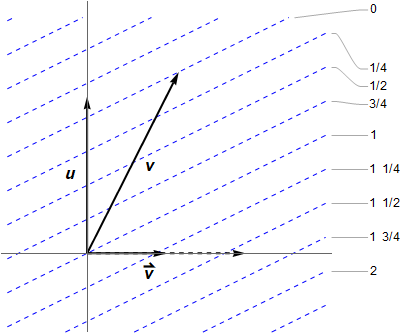
 is suggested by dotted blue lines, given at intervals of 1/4 for more resolution. These are orthogonal to the vector
  , so
, so  . One can show
  . Also
  , but I find it easier to think of:
  . These give the number of hyperplanes crossed by the unit axes vectors, then you can literally “connect the dots” since the 1-form is linear. In the figure
  , so
, so  . (As for the 3-gradient, it vanishes in the
  . It would be drawn as vertical lines, with corresponding vector pointing to the right.)
 adapted to the observer, meaning
  , and the
  vectors are orthogonal to
  . Then a purely spatial vector is spanned by the
  is the direction of steepest increase. We can mimic this mathematically by staying in 4 dimensions, but setting the “time” part to zero:
![\[^{(3)}d\Phi := d\Phi + \langle d\Phi,\mathbf u\rangle \mathbf u^\flat.\]](http://cmaclaurin.com/cosmos/wp-content/ql-cache/quicklatex.com-07b08d0090362be83cad765ee6df27e8_l3.png "Rendered by QuickLaTeX.com")
 ” to imply it vanishes in the observer’s time direction. This “3-gradient” is the projection of
 ![\[^{(3)}(d\Phi)^\sharp = (d\Phi)^\sharp + \langle d\Phi,\mathbf u\rangle \mathbf u.\]](http://cmaclaurin.com/cosmos/wp-content/ql-cache/quicklatex.com-f4c2ed9a3f4cd8007be9dd6c8b0433c1_l3.png "Rendered by QuickLaTeX.com")
 as usual. Note that on the subspace, the inverse metric coincides with the inverse 3-metric which has components
  , for
, for  . Equivalently, one can apply the spatial projector
  to either
  expresses the change in
 ![\[\nabla_\mu\Phi = (d\Phi)_\mu = \Phi_{,\mu} := \frac{\partial\Phi}{\partial x^\mu}.\]](http://cmaclaurin.com/cosmos/wp-content/ql-cache/quicklatex.com-527fbdf54171e7f1dad06b04f9c48a61_l3.png "Rendered by QuickLaTeX.com")
 ” is called the exterior derivative, and
  , on the manifold (MTW
  . Given some vector
  , the contraction:
![\[d\Phi(\mathbf Y) \equiv \langle d\Phi,\mathbf Y\rangle = Y^\mu\frac{\partial\Phi}{\partial x^\mu}\]](http://cmaclaurin.com/cosmos/wp-content/ql-cache/quicklatex.com-6b2759547d61189d856872022a7d65aa_l3.png "Rendered by QuickLaTeX.com")
 , both over the entire manifold and within a single tangent space. The spacing is
  .
. . This may be elegantly written
  has components
  , with
  just
just  . These contract to give unity. If we restrict to vectors spanned by
  and
and  , Schutz’ steepness comments apply. However
  is also a unit spacelike vector, where
  , hence crosses more intervals
  than the gradient vector does. Similarly for
  , the contraction with
  returns
  yields
  whenever
  . The angle brackets mean contraction using the metric, with indices appropriately raised or lowered. Another property is the gradient vector’s squared-norm equals the 1-form’s squared-norm, which also matches the number of contours crossed:
![\[\langle (d\Phi)^\sharp,(d\Phi)^\sharp\rangle = \langle d\Phi,d\Phi\rangle = \langle d\Phi,(d\Phi)^\sharp\rangle.\]](http://cmaclaurin.com/cosmos/wp-content/ql-cache/quicklatex.com-e96c271c1bf8871402d5b158d940c579_l3.png "Rendered by QuickLaTeX.com")
 , for which the hyperplanes are spanned by vectors satisfying
  . For many creative illustrations see MTW, including their “honeycomb” and “egg crate” analogies for 2-forms and 3-forms, and their Figure 4.5 for the 2-form
  . Finally, I previously
  , which give the rate of change of the scalar by proper time along a worldline.
 . The coordinate basis vectors are
  ,
,  , and
, and  , so for
  for example, this is the vector
  with components
  . Recall a connection
 ![\[\nabla_{\mathbf e_\mu}\mathbf e_\nu = \Gamma^\alpha_{\mu\nu}\mathbf e_\alpha,\]](http://cmaclaurin.com/cosmos/wp-content/ql-cache/quicklatex.com-27bb80f2a8f6f020a6a99a6a793f678f_l3.png "Rendered by QuickLaTeX.com")
 , this definition is interpreted as the derivative of the
  field, in the direction
 ![\[u^\mu = (A(t,r),B(t,r),0,0).\]](http://cmaclaurin.com/cosmos/wp-content/ql-cache/quicklatex.com-4d63f7a77a5c142d312b322bb6c5acf2_l3.png "Rendered by QuickLaTeX.com")
 or
or  and
and  -plane. As expected,
  does not vanish, even in these directions:
![\[\nabla_{C\partial_\theta + D\partial_\phi}\mathbf u = \Big(0,0,\frac{C B(t,r)}{r},\frac{D B(t,r)}{r}\Big).\]](http://cmaclaurin.com/cosmos/wp-content/ql-cache/quicklatex.com-4cde795af5f57b10bf8e03c23dbef917_l3.png "Rendered by QuickLaTeX.com")
 and
and  and
and  . These quantify how the radial
  and
and  , and keep the remaining Christoffel symbols, in order to remain as close as possible to the metric connection. This procedure is justified, because given a frame field, any choice of smooth functions
  yields a valid connection (Lee 2018
 ![\[\tilde\nabla_{\mathbf v}\mathbf u := \nabla_{\mathbf v}\mathbf u - \frac{1}{r} \big(\partial_\theta\otimes d\theta\otimes dr + \partial_\phi\otimes d\phi\otimes dr)(\mathbf v,\mathbf u).\]](http://cmaclaurin.com/cosmos/wp-content/ql-cache/quicklatex.com-0cb08921b118007ab2fa6f731a6a4fc0_l3.png "Rendered by QuickLaTeX.com")
 , where the angle brackets mean contraction of a 1-form and vector in this case. Intuitively, the parenthetical term just above is also a projection, returning only the angular part of the differentiation direction
  multiplier.
  returns the radial component
  .
. as required. The new connection is not symmetric, because
  and
and  remain non-vanishing. Hence the connection has “torsion”. I won’t write out its Riemann and Ricci tensors, but the scalar curvature is
  ! At face value this violates the Einstein field equations, for which the Ricci tensor (and hence the scalar curvature) always vanish in a vacuum, however Einstein’s equations use the Levi-Civita connection. Curiously, the value is precisely the scalar curvature for a 2-sphere.
 for which additionally
  . In the (somewhat) index-free expression:
![\[\bar\nabla_{\mathbf v}\mathbf u := \nabla_{\mathbf v}\mathbf u - \frac{2}{r} \big(\partial_\theta\otimes dr\,d\theta + \partial_\phi\otimes dr\,d\phi)(\mathbf v,\mathbf u),\]](http://cmaclaurin.com/cosmos/wp-content/ql-cache/quicklatex.com-b06eb486ce32cbf4d6dda1a77e2d4a97_l3.png "Rendered by QuickLaTeX.com")
 is the symmetric product, and analogously for
  . This connection has Ricci tensor equal to the metric in the
  , and vanishing elsewhere. Its scalar curvature is
  .
. . Hence
  . The same holds for
  and
and  , or scalar multiples thereof. I avoided this technicality in the interests of readability. This concern only applies to coordinate systems in which the metric is non-diagonal.
 tries to illustrate the various paths that reached us. The supernova was also featured in NASA’s